Download
1 / 25
250 likes | 351 Views
Explore how baroclinicity affects wind direction & magnitude in marine boundary layer, analyzing geostrophic shear & thermal winds. Evaluate baroclinicity's influence on cyclone genesis & intensification using buoy data & ECMWF variables.

E N D
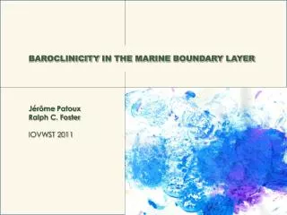
Baroclinicity in the marine boundary layer JérômePatoux Ralph C. Foster IOVWST 2011
PBL 101 STABLE Ta > Ts Ekman layer hp surface layer UNSTABLE Ts > Ta
horizontal temperature gradient cold thermal wind Ut T V/ z geostrophic shear warm “baroclinicity” In baroclinic conditions, the geostrophic shear is added to the BL shear, with an effect on both the magnitude and the direction of the wind throughout the profile.
Calculating surface winds from GFS SLP at the NOAA OPC (with Joe Sienkiewicz).
Calculating surface winds from GFS SLP at the NOAA OPC (with Joe Sienkiewicz).
Evaluating the impact of the baroclinicity associated with WBCs on the genesis and intensification of midlatitude cyclones. An example of two midlatitude cyclone tracks displayed over… SST 500-hPa heights
Vector correlations between QS 10m neutral-equivalent winds and NDBC buoy 10m neutral-equivalent winds (1999-2009).
NDBC buoy 44004 Calculate buoy 10m neutral-equivalent winds (COARE 3.0). Full QS period (1999-2009). Discard rain-flagged winds. Interpolate OSCAR currents. Interpolate closest-in-time ECMWF surface variables: Ta, Ts, Td, SLP. Calculate T.
V Ut Ut V
Conclusions Using one buoy (!) and 10 years of QS measurements (and interpolated ECMWF surface variables), we can reveal the modulation of the boundary layer profile by baroclinicity (i.e., thermal wind, or geostrophic shear). A modulation of the difference between neutral-equivalent buoy and QS wind speeds suggests that there remains an “error” in the QS 10m neutral-equivalent winds (~0.2-0.3 m/s) due to baroclinicity that is not resolved by the GMF and that cannot be corrected by a simple stratification correction.
Standard deviation of the directional differences between QS 10m neutral-equivalent winds and NDBC buoy 10m neutral-equivalent winds (1999-2009).
Standard deviation of the directional differences between QS 10m neutral-equivalent winds and NDBC buoy 10m neutral-equivalent winds (1999-2009). 46001 46002 46005 46006 46035 46059
Standard deviation of the directional differences between QS 10m neutral-equivalent winds and NDBC buoy 10m neutral-equivalent winds (1999-2009). 46001 46002 46005 46006 46035 46059 46066 51001 51002 51003 51004 51028
Standard deviation of the directional differences between QS 10m neutral-equivalent winds and NDBC buoy 10m neutral-equivalent winds (1999-2009). 46001 46002 46005 46006 46035 46059 46066 51001 51002 51003 51004 51028 +
Standard deviation of the directional differences between QS 10m neutral-equivalent winds and NDBC buoy 10m neutral-equivalent winds (1999-2009). 46001 46002 46005 46006 46035 46059 46066 51001 51002 51003 51004 51028 + + +