Download
1 / 16
180 likes | 751 Views
Suspended Load. Bed Load. Marine Boundary Layers Shear Stress Velocity Profiles in the Boundary Layer Laminar Flow/Turbulent Flow “Law of the Wall” Rough and smooth boundary conditions. Shear Stress. In cgs units: Force is in dynes = g * cm / s 2 Shear stress is in dynes/cm 2

E N D
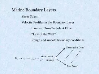
Suspended Load Bed Load Marine Boundary Layers Shear Stress Velocity Profiles in the Boundary Layer Laminar Flow/Turbulent Flow “Law of the Wall” Rough and smooth boundary conditions
Shear Stress In cgs units: Force is in dynes = g * cm / s2 Shear stress is in dynes/cm2 (N/m2 in MKS)
Z Y X Each plane has three components – i.e., for the x plane: For three dimensions: nine components What are the key components in the marine boundary layer?
XX, YY, ZZ component – is the pressure force, doesn’t act to move particles XZ, YZ component – the flow is not shearing in the z-direction (in the mean) XY, YX component – assume uniform flow (flow not rotating in the mean) End up with two components: , shear on the z-plane in x and y directions As we get close to the seabed and rotate into flow: τb
Simplest boundary layer case: Laminar Flow – smooth boundary no turbulence generated layers of fluid slipping past each other In this case: Z F h X “No-slip” condition
Deformation of fluid layers is at same rate for shearing force • linear velocity profile • Integrating: • Boundary conditions: • Description of velocity profile:
What force (or shear stress) was needed to pull plate A and create this velocity profile? Molecular viscosity of the fluid (resistance of the fluid to deformation) Provides transfer of momentum between adjacent fluid layers
Another way to think about shear stress: • Transfer of momentum perpendicular to the surface on which stress is applied. kinematic viscosity Velocity gradient Fluid momentum gradient Diffusion of momentum
Turbulent Flows • A random (statistically irregular) component added to the mean flow Dyer, 1986 Define u = instantaneous velocity u’ = random turbulent velocity ū = mean velocity u = ū + u’
NOTE! Beware of averaging time scale. Turbulent fluctuations follow a Gaussian distribution: Turbulence intensity can be described by the RMS fluctuation Frequency of occurrence Average of u’==0 u’ Turbulent eddies transfer momentum, much the same way as molecular diffusion, but at appreciably greater rates.
Transfer of momentum can be described by: • “eddy” viscosity - Az – transfer of momentum in z-direction • (note: in Wright, 1995 chapter) • Az >>
Eddy fluctuations and momentum transfer: • u’, v’, w’ - responsible for the transfer of momentum Middleton & Southard, 1984
Z ū • Parcel has lower momentum at z2 by ρΔu • flux of momentum: • w’•(ρΔu) • As z2 and z1 approach each other, • u2 - u1 = Δu u’ • flux of momentum: • w’•(ρu’) or u’w’ This rate of change of momentum represents the resistance to motion, or the shear stress, and averaged over time: Reynolds Stress
Since turbulent fluctuations difficult to characterize, simplifying assumptions can be made: • u’ u turbulent fluctuations are proportional to the mean flow • u’, v’, w’ are of similar magnitude Quadratic Stress Law
Summarize: Three ways to describe shear stress in the turbulent bottom boundary layer. • Eddy Viscosity • Reynolds Stress • Quadratic Stress Law