Classical Regression II
Classical Regression II. Lecture 8. The story so far. We learned how to compute least squares estimates We talked about the assumptions underlying the CLRM: 1) Y and e are random variables 2) X i is nonrandom (it’s given) 3) E( e i ) = E( e i |X i ) = 0

Classical Regression II
E N D
Presentation Transcript
Classical Regression II Lecture 8
The story so far... • We learned how to compute least squares estimates • We talked about the assumptions underlying the CLRM: 1) Y and e are random variables 2) Xi is nonrandom (it’s given) 3) E(ei) = E(ei|Xi) = 0 4) V(ei)= V(ei|Xi) = 2 5) Covariance (eiej) = 0 Clear about difference of ei and ei. Note that a and b (also denoted a^ and b^) are estimates of a and b; they are also random variables and have sampling distributions.
Today’s Plan • Inference with the classical linear regression model • Calculating the standard error • Calculating the t-ratio • Root-mean square error • 95% confidence intervals • ANOVA tables • ANOVA table: ANOVA stands for analysis of variance
X1 X2 X3 Variation around the regression line • iid, and assumed normal: Y3 Y1 Y2 X
Sum of Squares Identity • Let’s take one point, X1 and look at it graphically: Y X1
Sum of Squares Identity (2) • The Sum of Squares Identity is Total = Explained + Unexplained or
Sum of Squares Identity (3) reveals how much of the variation is explained by the regression line reveals how much of the variation is not explained by the regression line, or is left over • Notice that this is also equal to 2 reveals how much total variation there is • remember in a previous lecture we said that
How to calculate sum of squares • We can write the total sum of squares as • We’re given the Y values so we can compute • We can write the explained sum of squares as • Calculating the ESS: bSxy
How to calculate sum of squares (4) • We can calculate the unexplained variation (the unexplained sum of squares) as the difference between the total and the explained sum of squares: • Because we have to consider degrees of freedom when calculating each variance term, we divide the SSI by the corresponding degrees of freedom:
How to calculate sum of squares (5) • The residual variance of the regression line is • If we take the square root we get the root mean square error (root MSE):
Calculating test statistics • We can calculate test statistics from the sum of squares statistics • The variance of , the slope coefficient is • Where
Calculating test statistics (2) • The standard error of is • The variance of the intercept is • The standard error of is
Confidence intervals • Once we have the standard errors, we can do two things: • form a confidence interval • perform a hypothesis test • A confidence interval for b: • Where df in a bi-variate model is 2 • As with univariate cases, we can calculate a confidence interval for b in a bi-variate case
Hypothesis testing • Set up your null hypothesis and alternative • Determine the critical region - choose a significance level (a) • Using the relevant distribution, determine your critical (tabled) value (Za/2 , or ta/2 for the moment; Fdf1,df2 and cn soon). • For a given sample, compute the numeric value of the test statistic: Z*, t*, F* or c*. • Given the decision rule, determine whether to reject or not the null hypothesis.
Hypothesis testing (2) • For standard statistical packages, the null hypothesis is that the population parameter is zero, or Ho : b = 0 • Most of the time we only have a sample and an estimate , • we don’t know the actual population value • Sometimes the value of b is dictated by economic theory • in that case, a value will be imposed on b, such as b=1: Ho : b = 1
Hypothesis testing (3) • The standard t-ratio or t statistic is • So if the null hypothesis dictates b= 0, the t-ratio becomes
Example • Data on female earnings in Illinois {spreadsheet L8.xls} • The variables include earnings, earnings weights, and years of education • In this example, the first three columns represent the ‘population’. Select two samples of 30 at random from that population. First sample, create log earnings (ln Y). Note you can create means of X and Y. Multiply (ln Y) by years of education (XY). Square years of education (X2). Sum (XY) and Sum (X2). Provides all the statistics you need to calculate the least squares line
Example (2) • I have also included an example of how to use Excel’s LINEST to calculate the regression line • On the web you’ll find some output from Stata using the population and sample regressions from the Illinois data. Try the LINEST function and check that your output agrees with the output from Stata • Let’s look at a graph of the sample and popluation regression lines
Example (3) • From the spreadsheet we calculated the following: Sample size : n=30 • We use these numbers to calculate
Example (4) • And to calculate • Compare our estimates with the Stata output • Now let’s use the numbers from the spreadsheet to calculate the regression line variance
Example (5) • The variance of is • Thus the standard error of is
Example (6) • We can calculate a confidence interval for b: • For a 95% confidence interval, b is bounded between 0.120 < b < 0.350
Example (7) • Now the hypothesis test: The Stata output gives a t-ratio of 4.06. Our null and alternative hypotheses are Ho: b = 0 Ho: b 0 • Our t statistic: • Since |t| > t/2df,, we reject the null hypothesis. • Thus, at a 95% confidence interval, the estimate does not equal zero
A word on modeling • The model we’ve been using is Y = a+bX • In our spreadsheet example, our model is lnY = a + bX • This suggests an underlying model of Y = ea+bX • Sometimes it is better to take logs of variables to make the relationship between Y and X linear • Because of outliers, the underlying relationship will sometimes look more like an upward sloping curve • Logging the earnings and then comparing it it years of education gives you a far more linear relationship - it does not change your conclusions
A word on modeling (2) • We are asking the question: • What is the increase in earnings for an additional year of education? • It is the differential • More simply we can write
A word on modeling (3) • The difference between X1 and X2 is a discreet change in years of education, so the difference will be one • So we can write: • On the spreadsheet, calculate an additional year of school: % of Y = e0.235 - 1 = approximately 26% Enter into Excel: =exp(0.235)-1 • So in a semi-log equation is lnY = + X % of Y