Download

1 / 12
120 likes | 261 Views
Classical regression review. Important equations Functional form of the regression Regression coefficients Standard error Coefficient of determination Variance of coefficients Variance of regression Variance of prediction. Practice example. Example problem. % Data

E N D
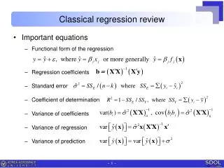
Classical regression review • Important equations • Functional form of the regression • Regression coefficients • Standard error • Coefficient of determination • Variance of coefficients • Variance of regression • Variance of prediction
Practice example • Example problem % Data y=[0.95, 1.08, 1.28, 1.23, 1.42, 1.45]'; x=[0 0.2 0.4 0.6 0.8 1.0]'; be = [0.9871 0.4957] se = 0.0627 R = 0.9162 sebe = [0.0454 0.0750] corr= -0.8257 Conf. interval = red line Pred. interval = magenta line
Bayesian analysis of classical regression • Remark • Classical regression is turned into the Bayesian: unknown coefficients b are estimated conditional on the observed data set (x,y). • If non-informative prior for b, solution is the same as the classical one.If there exist certain priors, however, there is no closed form solution. • Like we did before, we can practice Bayesian and validate results using the classical solution, in case of non-informative prior. • Statistical definition of the data • Assuming normal distribution of the data with the mean at regression equation, the data distribution is expressed as • Parameters to be estimated • Regression coefficients b=[b1,b2] ( something like m) and variance s2.
Joint posterior pdf of b, s2 • Non-informative prior • Likelihood to observe the data y • Joint posterior pdf of b=[b1,b2], s2(this is 3 parameters problem) • Compare with posterior pdf of normal distribution parameters m,s2
Joint posterior pdf of b, s2 • Analytical procedure • Factorization • Marginal pdf of s2 • Conditional pdf of b • Posterior predictive distribution • Sampling method based on factorization approach • Draw random s2 from inverse- c2 distribution. • Draw random b from conditional pdfb|s2. • Draw predictive ỹ at a new point using the expression ỹ|y.
Practice example • Joint posterior pdf of b, s2 • Data • This is function of 3 parameters.In order to draw the shape of the pdf, let’s assume s = 0.06.Max location of be = [b1 b2] is near [1 0.5] which agrees with true values. where X=[ones(n,1) x]; y=[0.95, 1.08, 1.28, 1.23, 1.42, 1.45]'; x=[0 0.2 0.4 0.6 0.8 1.0]';
Practice example • Sampling by MCMC • Using N=1e4, starting from b=[0;0] and s=1, as we iterate MCMC, we get convergence of b and s. At the initial stage, however, samples should be discarded. This is called Burn-in. • The max likelihood of b is found near [1;0.5], and of s near 0.06, which agree with the true values.
Practice example • Sampling by MCMC • Using N=1e4, MCMC is repeated ten times.The variances of the results are favorably small, which shows that the distribution can be accepted as the solution. * * * * * * * * * * * * * * *
Practice example • Sampling by MCMC • Different value of w for proposal pdf leads to convergence failure.
Practice example • Sampling by MCMC • Different starting point of b may be suggested to check convergence and whether we get the same result.
Practice example • Posterior analysis • Posterior distribution of regression: using samples of B1 & B2, samples of ym are generated, where ym = B1+B2*x. • Blue curve is the mean of ym. • Red curves are the confidence bounds of ym. (2.5%, 97.5% of the samples.) • Posterior predictive distribution: using samples of ym and S, samples of predicted y are generated, i.e., yp ~ N(ym,s2).
Confidence vsprediction interval • Classical regression • Confidence interval comes from variance of regression • Prediction interval comes from variance of prediction • Bayesian approach of regression • Confidence interval comes from Posterior distribution of regression. • Predictive interval comes from Posterior predictive distribution. • Bayesian approach of normal distribution • Confidence interval comes fromt-distribution with n-1 dof wheremean ȳ and variance s2/n. • Predictive interval comes from t-distribution with n-1 dof wheremean ȳ and variance s2/n + s2.