AUTOCORRELATION OR SERIAL CORRELATION

1. AUTOCORRELATION OR SERIAL CORRELATION

2. Serial Correlation (Chapter 11.1) • Now let’s relax a different Gauss–Markov assumption. • What if the error terms are correlated with one another? • If I know something about the error term for one observation, I also know something about the error term for another observation. • Our observations are NOT independent!

3. Serial Correlation (cont.) • Serial Correlation frequently arises when using time series data (so we will index our observations with t instead of i) • The error term includes all variables not explicitly included in the model. • If a change occurs to one of these unobserved variables in 1969, it is quite plausible that some of that change will still be evident in 1970.

4. Serial Correlation (cont.) • In this lecture, we will consider a particular form of correlation among error terms. • Error terms are correlated more heavily with “nearby” observations than with “distant” observations. • E.g., cov(e1969,e1970) > cov(e1969,e1990)

5. Serial Correlation (cont.) • For example, inflation in the United States has been positively serially correlated for at least a century. We expect above average inflation in a given period if there was above average inflation in the preceding period. • Let’s look at DEVIATIONS in US inflation from its mean from 1923–1952 and from 1973–2002. There is greater serial correlation in the more recent sample.

6. Figure 11.1 U.S. Inflation’s Deviations from Its Mean

7. Serial Correlation: A DGP • We assume that covariances depend only on the distance between two time periods, |t-t’|

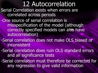
8. OLS and Serial Correlation (Chapter 11.2) • The implications of serial correlation for OLS are similar to those of heteroskedasticity: • OLS is still unbiased • OLS is inefficient • The OLS formula for estimated standard errors is incorrect • “Fixes” are more complicated

9. OLS and Serial Correlation (cont.) • As with heteroskedasticity, we have two choices: • We can transform the data so that the Gauss–Markov conditions are met, and OLS is BLUE; OR • We can disregard efficiency, apply OLS anyway, and “fix” our formula for estimated standard errors.

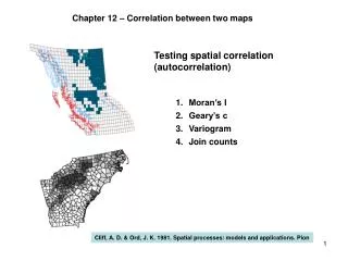
10. Testing for Serial Correlation Correlograms & Q-statistics View/residual tests/correlogram-q If there is no autocorrelation in the residuals, the auto and partial correlations at all lags should be nearly zero and Q-statistic should be insignificant with larger p-values

11. Durbin–Watson Test • How do we test for serial correlation? • James Durbin and G.S. Watson proposed testing for correlation in the error terms between adjacent observations. • In our DGP, we assume the strongest correlation exists between adjacent observations.

12. Durbin–Watson Test (cont.) • Correlation between adjacent disturbances is called “first-order serial correlation.” • To test for first-order serial correlation, we ask whether adjacent e ’s are correlated. • As usual, we’ll use residuals to proxy for e • The trick is constructing a test statistic for which we know the distribution (so we can calculate the probability of observing the data, given the null hypothesis).

13. Durbin–Watson Test (cont.) • We end up with a somewhat opaque test statistic for first-order serial correlation

14. Durbin–Watson Test (cont.) • In large samples, approximately estimates the covariance between adjacent error terms. If there is no first-order serial correlation, this term will collapse to 0.

15. Durbin–Watson Test (cont.) • When the Durbin–Watson statistic, d, gives a value far from 2, then it suggests the covariance term is not 0 after all • i.e., a value ofd far from 2 suggests the presence of first-order serial correlation • d is bounded between 0 and 4

16. Durbin–Watson Statistic • VERY UNFORTUNATELY, the exact distribution of the dstatistic varies from application to application. • FORTUNATELY, there are bounds on the distribution.

17. Durbin–Watson Statistic (cont.) • There are TWO complications in applying the Durbin–Watson statistic: • We do not know the exact critical value, only a range within which the critical value falls. • The rejection regions are in relation to d = 2, not d = 0.

18. TABLE 11.2 The Durbin–Watson Test

19. Figure 11.3 Durbin–Watson Lower and Upper Critical Values for n = 20 and a Single Explanator, = 0.5 (Panel B)

20. TABLE 11.1 Upper and Lower Critical Values for the Durbin–Watson Statistic (5% significance level)

21. Durbin–Watson Test • The Durbin–Watson test has three possible outcomes: reject, fail to reject, or the test is uncertain. • The Durbin–Watson test checks ONLY for first-order serial correlation.

22. Checking Understanding • Suppose we are conducting a 2-sided Durbin–Watson test with n = 80 and 1 explanator. For the 0.05 significance level, dl= 1.61 dh= 1.66 • Would you a) reject the null, b) fail to reject the null, or c) is the test uncertain, for: • i) d= 0.5; ii) d = 1.64; iii) d = 2.1; and iv) d = 2.9?

23. Checking Understanding (cont.) dl= 1.61 dh= 1.66 • Would you reject the null, fail to reject the null, or is the test uncertain, for: • i) d = 0.5: d < dl , so we reject the null. • ii) d = 1.64: dl<d < dh , so the test is uncertain. • iii) d= 2.1: dh< d < (4-dh), so we fail to reject. • iv) d= 2.9: d > (4-dl), so we reject the null.

24. Durbin–Watson Test • Suppose we find serial correlation. OLS is unbiased but inefficient.

25. Durbin–Watson Test (cont.) • Instead of using OLS, can we construct a BLUE Estimator? • First, we need to specify our DGP.

26. One Serial Correlation DGP

27. BLUE Estimation (cont.)

28. BLUE Estimation (cont.) • To get rid of the serial correlation term, we must algebraically manipulate the DGP. • Notice that

29. BLUE Estimation (cont.) • If we regress (Yt -rYt-1) against a constant and (Xt- rXt-1), we can estimate b1 in a model that meets the Gauss–Markov assumptions.

30. BLUE Estimation (cont.) • After transforming the data, we have the following DGP

31. BLUE Estimation (cont.) • With the transformed data, OLS is BLUE. • This approach is also called GLS. • There are two problems: • We cannot include the first observation in our regression, because there is no Y0 orX0to subtract. Losing an observation may or may not be a problem, depending on T • We need to know r

32. Checking Understanding • What Gauss–Markov assumption is violated if we restore the first observation?

33. Checking Understanding (cont.) • The first observation’s error term is not correlated with any other error terms; this DGP does not suffer from serial correlation.

34. Checking Understanding (cont.) • The error term of the first observation has a different variance than the other error terms. • This DGP suffers from heteroskedasticity.

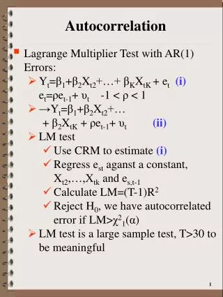
35. LM Test • If your model included a lagged dependent variable on the right hand side then DW is not an appropriate test for serial correlation • Using OLS on such a regression results in biased and inefficient coefficients

36. Use Breusch-Godfrey Lagrange Multiplier test for general high order auto test The test statistic has an asymptotic χsquared (Chi-squared distribution) View residual test serial corr LM

37. BLUE Estimation (cont.) • This FGLS procedure is called the Cochrane–Orcutt estimator.