Scatter Diagrams & Correlation/Regression Analysis

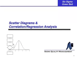
Sigma Quality Management -6 -4 -2 0 2 4 6 Scatter Diagrams & Correlation/Regression Analysis

Scatter/Correlation Situations • Increasing the pressure in the plastic injection molds reduces the number of defective parts. • Increasing temperature and catalyst concentration improves the yield of the chemical reaction.

Scatter Diagrams Gas Mileage (MPG) 26 Driving Speed (MPH) 20 35 75

Tubing - Copper Content Measurement (Portable vs. Laboratory Models) Copper Content (Portable Sampler) Copper Content (Laboratory Spectrometer) Surrogate Indicators

Y-max 3” Y-min X-min X-max 3” Construction 1. Define the two variables that you think are correlated. Causative (or independent) variable vs. effect (or dependent variable). 2. Collect the data in pairs. 3. Draw a horizontal and vertical axis. Label the horizontal axis with the name of the independent (or causative) variable, the vertical axis with the dependent variable (or effect). 4. Scale these axes so that both the independent and dependent variables’ range is about the same distance.

Construction • Plot the data pairs as points on the scatter diagram. If there are identical points, draw a circle around the first one plotted. • Make sure you put a title and label on the scatter diagram. Include the date(s) the data was collected and who prepared the diagram. 7. Interpret the scatter diagram for possible correlation between the variables.

Scatter Interpretation

0 -1.0 +1.0 Correlation Coefficient Values “Perfect” Negative Correlation “Perfect” Positive Correlation No Correlation The Correlation Coefficient

Correlation vs. Cause & Effect • The population of Paris was positively correlated to the number of stork nests in the city. • The homicide rate in Chicago is positively correlated to the sales of ice cream by street vendors. • At one time, the Dow Jones stock market index was positively correlated to the height of women’s hemlines. • Your Examples?

Regression Models y = mx + b y m = Rise Run Rise Run b 0 x 0

Residuals – Basis for Model Fitting y Error y = mx + b Error ei = yi - (mxi+b) x

Simple Linear Regression - Steps 1. Collect the data pairs, or obtain them from the raw data used to create the Scatter Diagram. 2. Calculate the average of the dependent variable and independent variable:

Simple Linear Regression - Steps 3. Calculate the estimate of the slope of the regression line (note that we use the “hat” symbol () to show that we are estimating the true population slope):

Simple Linear Regression - Steps 4. Finally, calculate the estimate of the y-intercept, : 5. Plot the regression line on the scatter diagram. Visually check the line to see if it is a good fit and that no calculation errors were made.

Checking the Regression Model Residuals Analysis: • X, mR Control Chart of Residuals • Histogram or Normal Probability Plots • Scatter Diagram – Residuals vs. Independent Variable

Interpolation Dangers Y POSSIBLE RELATIONSHIPS “BEYOND THE MAX” X XMin XMax

Confidence & Prediction Bounds y y = mx + b Confidence Bound for Regression Line Confidence Bound for Points x

Scatter Diagrams & Correlation/Regression Analysis