Understanding Correlation and Regression: Key Concepts and Applications
This article provides an in-depth exploration of correlation and regression analysis, focusing on scatter plots to visualize relationships between two data series. We discuss sample covariance, the correlation coefficient, and the implications of outliers and spurious correlations. The article also covers the basics of linear regression, focusing on assumptions, parameter estimation, and regression output metrics such as standard errors and the coefficient of determination. Learn how these statistical tools can help in analyzing relationships and making data-driven decisions.

Understanding Correlation and Regression: Key Concepts and Applications
E N D
Presentation Transcript
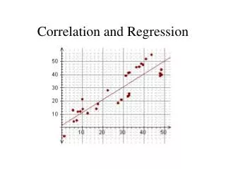
Scatter plots A scatter plot is a graph that shows the relationship between the observations for two data series in two dimensions. Scatter plots are formed by using the data from two different series to plot coordinates along the x- and y-axis, where one element of the data series forms the x-coordinate and the other the y-coordinate. Linear Nonlinear
Sample covariance Recall that covariance is the weighted average of the cross-product of each variable’s departure from its mean. Sample covariance is calculated by using the same process as sample variance; however, rather than squaring the deviation of each observation from its mean, we take the product of two different variables’ deviations from their respective means.
Sample covariance Focus On: Calculations Lending rates and current borrower burden are generally believed to be related. The following data cover the debt-to-income ratio for 10 borrowers and the interest rate they are being charged on five-year loans. What is the sample covariance between loan rate (Y) and debt-to-income ratio (X)?
Correlation Coefficient The correlation coefficient measures the extent and direction of a linear association between two variables. If the sample covariance is denoted as sx,y, then the sample correlation coefficient is the sample covariance divided by each sample standard deviation or Continuing with our example, the sample correlation coefficient is then From this result, we can conclude that there is a strong linear relationship between the debt-to-income ratio of the borrowers and the loan rate they are charged. Furthermore, we can conclude that the relationship has a positive sign, indicating that an increase in the debt-to-income ratio is associated with a higher loan rate.
Limitations of correlation analysis Focus On: Outliers Outliers are small numbers of observations with extreme values vis-à-vis the rest of the sample. Noise or news? Should we include them or discard them? Outliers can create the appearance of a linear relationship when there isn’t one OR create the appearance of no linear relationship when there is one.
Spurious correlation Spurious correlation is estimated correlation that arises because of the estimating process, not because of a fundamental underlying linear association. Potential sources of spurious correlation: Correlation between two variables that reflects chance relationships in a particular dataset. Correlation induced by a calculation that mixes each of two variables with a third. Correlation between two variables arising not from a direct relationship between them but from their relationship to a third variable.
Correlation coefficients Focus On: Hypothesis Tests Recall from Chapter 7 that we can test the value of a correlation coefficient as compared with the true correlation coefficient parameter using the test statistic: Returning to our earlier example, we can test whether the correlation between the debt-to-income ratio and the loan rate is zero at a 95% confidence level. Formulate hypothesis H0: r = 0versus Ha: r ≠ 0 (a two-tailed test) Identify appropriate test statistic (see above) Specify the significance level 0.05 leading to a critical value of 2.306 Collect data and calculate test statistic Make the statistical decision Reject the null because 4.134 > 2.306 Statistically The correlation between the debt-to-income ratio and the loan rate is nonzero.Economically Higher debt-to-income ratios are associated with higher loan rates.
The Basics of Linear regression Linear regression allows us to describe one variable as a linear function of another variable. The independent variable (Xi) is the variable you are using to explain changes in the dependent variable (Yi), the variable you are attempting to explain. The linear regression estimation process chooses parameter estimates to minimize the sum of the squared departures of the predicted values from the observed values. b0 is known as the intercept and b1 is known as the slope coefficient. If the value of the independent variable increases by one unit, the value of the dependent variable changes by b1 units. e { b1 = 0.78 b0 = 0.026
Assumptions underlying linear regression The relationship between the dependent variable, Y, and the independent variable, X, is linear in the parameters b0 and b1. The independent variable, X, is not random. The expected value of the error term is 0 E(ε) = 0. The variance of the error term is the same for all observations. The error term, ε, is uncorrelated across observations. Consequently, E(εi,εj) = 0 for all i not equal to j. The error term, ε, is normally distributed.
The Basics of Linear regression Focus On: Regression Output
Standard error of the estimate The standard error of the estimate gives us a measure of the goodness of fit for the relationship.
Coefficient of determination The coefficient of determination is the portion of variation in the dependent variable explained by variation in the independent variable(s). Total variation = Unexplained variation + Explained variation; therefore, we can calculate it two ways. Square the correlation coefficient when we have one dependent and one independent variable. We can use the above relationship to determine the unexplained portion of the total variation as the sum of the squared prediction errors divided by the total variation in the dependent variable when we have more than one independent variable. Because we have one independent and one dependent variable in our regression, the coefficient of determination is 0.82532 = 0.6811. The debt-to-income ratio explains 68.11% of the variation in loan rate.
Regression coefficients Focus On: Calculations When we calculate the confidence interval for a regression coefficient, we can use the estimated coefficient, the standard error of that coefficient, and the distribution of the coefficient estimate (in this case, a t-distribution) to estimate a confidence interval as For a 95% confidence interval of our estimated slope coefficient of 0.7774, the confidence interval would be or
Regression coefficients Focus On: Hypothesis Testing Alternatively, we could test the hypothesis that the true population slope coefficient is zero. Formulate hypothesis H0: b1 = 0versus Ha: b1 ≠ 0 (a two-tailed test) Identify appropriate test statistic Specify the significance level 0.05 leading to a critical value of 2.3060 Collect data and calculate test statistic Make the statistical decision Reject the null because 4.1538 > 2.3060
Regression coefficients Focus On: Interpretation 6. Interpret the results of the test. Statistically The coefficient estimate for the slope of the relationship is nonzero. Economically A unit increase in the debt-to-income ratio leads to a 0.7774 unit increase in the loan rate. In other words, an increase of 1% in the debt-to-income ratio leads to a 77.74 basis point increase in the loan rate charged.
Prediction and Linear regression Focus On: Calculating Predicted Values Continuing with our example, we can calculate predicted values for our dependent variable given our estimated regression model and values for our independent variable. If we want to predict the value of a loan rate for a borrower with a debt-to-income ratio of 18%, we substitute our estimated coefficients and a value of X = 0.18 to get For our estimated relationship, a borrower with an 18% debt-to-income ratio would be expected to have a 16.58% loan rate.
Prediction and Linear regression Focus On: Calculations Just as we can estimate a confidence interval for our coefficients, we can also estimate a confidence interval for our predicted (forecast) values. But we must also account for the estimation error in our coefficient estimates: Using the coefficient estimates and our predicted value from the prior slide, we determine a 95% confidence interval for our prediction:
Analysis of variance Known as ANOVA, this process enables us to divide the total variability in the dependent variable into components attributable to different sources. ANOVA allows us to estimate the usefulness of an independent variable or variables in explaining the variation in the dependent variable. We do so using a test that determines whether the estimated coefficients are jointly zero. The ratio of the mean regression sum of squares to the mean squared error follows an F-distribution with 1 and n – 2 degrees of freedom. For a single independent variable, this is expressed as SSE = the sum of the squared errors (residuals) and RSS = the sum of the squared deviations of the predicted values from the mean value of the dependent variable or
Analysis of variance Focus On: Calculations For our example, with a single independent variable, we can test the overall significance of the estimated relationship. Formulate hypothesis H0: all b = 0versus Ha: all b ≠ 0 Identify appropriate TS Specify the significance level 0.05 leading to CV = 5.3176 Collect data (see above) and calculate test statistic 5. Make the statistical decision Reject the null 6. Statistically at least one b is non-zero Economically the specified relationship has valid explanatory power
Limitations of regression analysis Parameter instability occurs when regression relationships change over time. This instability generally occurs when the underlying population from which the sample is drawn has changed fundamentally in some way. Example: regime shifts in regulatory or monetary policy Public knowledge of the relationships may decrease or eliminate their usefulness. Violation of the underlying assumptions makes hypothesis tests and prediction intervals invalid, and we may not be certain as to whether the assumptions have been violated.
Summary We are often interested in knowing the extent of the relationship between two or more financial variables. We can assess this relationship in several ways, including correlation, which measures the degree to which two variables move together, and linear regression, which describes at a more fundamental level the nature of any linear relationship between two variables. We can combine hypothesis testing from the prior chapter with linear regression and correlation to test beliefs about the nature and extent of relationships between two or more variables.