Download
1 / 35
350 likes | 372 Views
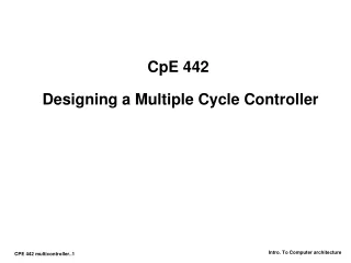
CpE 442 Designing a Multiple Cycle Controller. Outline of Today’s Lecture. Recap (5 minutes) Review of FSM control (15 minutes) From Finite State Diagrams to Microprogramming (25 minutes) ABCs of microprogramming (25 minutes). Review of a Multiple Cycle Implementation.

E N D
Outline of Today’s Lecture • Recap (5 minutes) • Review of FSM control (15 minutes) • From Finite State Diagrams to Microprogramming (25 minutes) • ABCs of microprogramming (25 minutes)
Review of a Multiple Cycle Implementation • The root of the single cycle processor’s problems: • The cycle time has to be long enough for the slowest instruction • Solution: • Break the instruction into smaller steps • Execute each step (instead of the entire instruction) in one cycle • Cycle time: time it takes to execute the longest step • Keep all the steps to have similar length • This is the essence of the multiple cycle processor • The advantages of the multiple cycle processor: • Cycle time is much shorter • Different instructions take different number of cycles to complete • Load takes five cycles • Jump only takes three cycles • Allows a functional unit to be used more than once per instruction
ALU 32 ALU Control 32 Review: Instruction Fetch Cycle, In the Beginning • Every cycle begins right AFTER the clock tick: • mem[PC] PC<31:0> + 4 Clk One “Logic” Clock Cycle You are here! PCWr=? PC 32 MemWr=? IRWr=? 32 32 RAdr Clk 4 32 Ideal Memory Instruction Reg WrAdr 32 Dout Din 32 ALUop=? 32 Clk
ALU 32 ALU Control 32 Review: Instruction Fetch Cycle, The End • Every cycle ends AT the next clock tick (storage element updates): • IR <-- mem[PC] PC<31:0> <-- PC<31:0> + 4 Clk One “Logic” Clock Cycle You are here! PCWr=1 PC 32 MemWr=0 IRWr=1 32 00 32 RAdr Clk 4 32 Ideal Memory Instruction Reg 32 WrAdr Dout Din ALUOp = Add 32 32 Clk
Target 32 0 Mux 0 Mux 1 ALU 0 1 Mux 32 1 ALU Control Mux 1 0 << 2 Extend 16 Putting it all together: Multiple Cycle Datapath PCWr PCWrCond PCSrc BrWr Zero ALUSelA IorD MemWr IRWr RegDst RegWr 1 Mux 32 PC 0 Zero 32 Rs Ra 32 RAdr 5 32 Rt Rb busA 32 Ideal Memory 32 Instruction Reg Reg File 5 32 4 Rt 0 Rw 32 WrAdr 32 1 32 Rd Din Dout busW busB 32 2 32 3 Imm 32 ALUOp ExtOp MemtoReg ALUSelB
Ifetch ALUOp=Add 1: PCWr, IRWr x: PCWrCond RegDst, Mem2R Others: 0s Target 32 0 Mux 0 Mux 1 ALU 1 32 ALU Control Instruction Fetch Cycle: Overall Picture PCWr=1 PCWrCond=x PCSrc=0 BrWr=0 Zero ALUSelA=0 IorD=0 MemWr=0 IRWr=1 1 Mux 32 PC 0 Zero 32 32 RAdr 32 busA Ideal Memory 32 Instruction Reg 32 4 0 32 WrAdr 32 1 32 Din Dout busB 32 2 32 3 ALUSelB=00 ALUOp=Add
Rfetch/Decode ALUOp=Add 1: BrWr, ExtOp ALUSelB=10 x: RegDst, PCSrc IorD, MemtoReg Others: 0s Target 32 0 Mux 0 Mux 1 ALU 0 1 Mux 1 ALU Control << 2 Extend Register Fetch / Instruction Decode (Continue) • busA <- Reg[rs] ; busB <- Reg[rt] ; • Target <- PC + SignExt(Imm16)*4 PCWr=0 PCWrCond=0 PCSrc=x BrWr=1 Zero ALUSelA=0 IorD=x MemWr=0 IRWr=0 RegDst=x RegWr=0 1 Mux 32 PC 0 Zero 32 Rs Ra 32 RAdr 5 32 Rt Rb busA 32 Ideal Memory 32 Instruction Reg Reg File 5 32 4 Rt 0 Rw 32 WrAdr 32 1 32 Rd 32 Din Dout busW busB 32 2 32 3 Control Beq Op Rtype Imm 6 ALUSelB=10 Ori Func Memory 6 16 32 ALUOp=Add : ExtOp=1
RExec 1: RegDst ALUSelA ALUSelB=01 ALUOp=Rtype x: PCSrc, IorD MemtoReg ExtOp Target 32 0 Mux 0 Mux 1 ALU 0 1 Mux 1 ALU Control Mux 1 0 << 2 Extend 16 R-type Execution • ALU Output <- busA op busB PCWr=0 PCWrCond=0 PCSrc=x BrWr=0 Zero ALUSelA=1 IorD=x MemWr=0 IRWr=0 RegDst=1 RegWr=0 1 Mux 32 PC 0 Zero 32 Rs Ra 32 RAdr 5 32 Rt Rb busA 32 Ideal Memory 32 Instruction Reg Reg File 5 32 4 Rt 0 Rw 32 WrAdr 32 1 32 Rd 32 Din Dout busW busB 32 2 32 3 Imm 32 ALUOp=Rtype ExtOp=x MemtoReg=x ALUSelB=01
Rfinish ALUOp=Rtype 1: RegDst, RegWr ALUselA ALUSelB=01 x: IorD, PCSrc ExtOp Target 32 0 Mux 0 Mux 1 ALU 0 1 Mux 32 1 ALU Control Mux 1 0 << 2 Extend 16 R-type Completion • R[rd] <- ALU Output PCWr=0 PCWrCond=0 PCSrc=x BrWr=0 Zero ALUSelA=1 IorD=x MemWr=0 IRWr=0 RegDst=1 RegWr=1 1 Mux 32 PC 0 Zero 32 Rs Ra 32 RAdr 5 32 Rt Rb busA 32 Ideal Memory 32 Instruction Reg Reg File 5 32 4 Rt 0 Rw 32 WrAdr 32 1 32 Rd Din Dout busW busB 32 2 32 3 Imm 32 ALUOp=Rtype ExtOp=x MemtoReg=0 ALUSelB=01
Outline of Today’s Lecture • Recap (5 minutes) • Review of FSM control (15 minutes) • From Finite State Diagrams to Microprogramming (25 minutes) • ABCs of microprogramming (25 minutes)
Overview of Next Two Lectures • Control may be designed using one of several initial representations. The choice of sequence control, and how logic is represented, can then be determined independently; the control can then be implemented with one of several methods using a structured logic technique. Initial Representation Finite State Diagram Microprogram Sequencing Control Explicit Next State Microprogram counter Function + Dispatch ROMs Logic Representation Logic Equations Truth Tables Implementation Technique PLA ROM “hardwired control” “microprogrammed control”
Ifetch Rfetch/Decode BrComplete ALUOp=Add 1: PCWr, IRWr ALUOp=Add ALUOp=Sub x: PCWrCond 1: BrWr, ExtOp ALUSelB=01 RegDst, Mem2R ALUSelB=10 x: IorD, Mem2Reg Others: 0s RegDst, ExtOp x: RegDst, PCSrc IorD, MemtoReg 1: PCWrCond ALUSelA Others: 0s PCSrc RExec 1: RegDst ALUSelA ALUOp=Or ALUSelB=01 1: ALUSelA ALUOp=Rtype ALUSelB=11 x: PCSrc, IorD MemtoReg x: MemtoReg ExtOp IorD, PCSrc Rfinish 1: ALUSelA ALUOp=Rtype ALUOp=Or RegWr, ExtOp 1: RegDst, RegWr MemtoReg x: IorD, PCSrc ALUselA ALUSelB=11 ALUSelB=11 ALUSelB=01 ALUOp=Add 1: ALUSelA x: IorD, PCSrc x: PCSrc RegWr ExtOp IorD Initial Representation: Finite State Diagram 0 1 8 beq 2 AdrCal 1: ExtOp ALUSelA ALUSelB=11 lw or sw ALUOp=Add x: MemtoReg Ori PCSrc 10 Rtype lw sw OriExec 3 6 5 SWMem LWmem 1: ExtOp ALUSelA, IorD 1: ExtOp MemWr ALUSelB=11 ALUSelA ALUOp=Add ALUSelB=11 x: MemtoReg ALUOp=Add PCSrc x: PCSrc,RegDst 11 MemtoReg OriFinish 7 4 LWwr
Opcode Sequencing Control: Explicit Next State Function O u t p u t s Control Logic • Next state number is encoded just like datapath controls Multicycle Datapath Inputs State Reg
Logic Representative: Logic Equations • Alternatively, prior state & condition • S4, S5, S7, S8, S9, S11 -> State0 • _________________ -> State 1 • _________________ -> State 2 • State2 & op = lw -> State 3 • _________________-> State 4 • State2 & op = sw -> State 5 • _________________ -> State 6 • State 6 -> State 7 • _________________ -> State 8 • State1 & op = jmp -> State 9 • _________________ -> State 10 • State 10 -> State 11 • Next state from current state • State 0 -> State1 • State 1 -> S2, S6, S8, S10 • State 2 ->__________ • State 3 ->__________ • State 4 ->State 0 • State 5 -> State 0 • State 6 -> State 7 • State 7 -> State 0 • State 8 -> State 0 • State 9-> State 0 • State 10 -> State 11 • State 11 -> State 0
S3 S2 S1 S0 NS3 NS2 NS1 NS0 Implementation Technique: Programmed Logic Arrays • Each output line the logical OR of logical AND of input lines or their complement: AND minterms specified in top AND plane, OR sums specified in bottom OR plane Op5 R = 000000 beq = 000100 lw = 100011 sw = 101011 ori = 001011 jmp = 000010 Op4 Op3 Op2 Op1 Op0 0 = 0000 1 = 0001 2 = 0010 3 = 0011 4 = 0100 5 = 0101 6 = 0110 7 = 0111 8 = 1000 9 = 1001 10 = 1010 11 = 1011
S3 S2 S1 S0 NS3 NS2 NS1 NS0 Implementation Technique: Programmed Logic Arrays • Each output line the logical OR of logical AND of input lines or their complement: AND minterms specified in top AND plane, OR sums specified in bottom OR plane lw = 100011 sw = 101011 R = 000000 ori = 001011 beq = 000100 jmp = 000010 Op5 Op4 Op3 Op2 Op1 Op0 0 = 0000 1 = 0001 2 = 0010 3 = 0011 4 = 0100 5 = 0101 6 = 0110 7 = 0111 8 = 1000 9 = 1001 10 = 1010 11 = 1011
Multicycle Control • Given numbers of FSM, can turn determine next state as function of inputs, including current state • Turn these into Boolean equations for each bit of the next state lines • Can implement easily using PLA • What if many more states, many more conditions? • What if need to add a state?
Outline of Today’s Lecture • Recap (5 minutes) • Review of FSM control (15 minutes) • From Finite State Diagrams to Microprogramming • ABCs of microprogramming (25 minutes)
Next Iteration: Using Sequencer for Next State • Before Explicit Next State: Next try variation 1 step from right hand side Initial Representation Finite State Diagram Microprogram Sequencing Control Explicit Next State Microprogram counter Function + Dispatch ROMs Logic Representation Logic Equations Truth Tables Implementation Technique PLA ROM “hardwired control” “microprogrammed control”
State Reg Opcode Sequencer-based control unit Control Logic To Multicycle Data path Control Signals Outputs Inputs Types of “branching” • Set state to 0 • Dispatch (state 1 & 2) • Use incremented state number 1 MicroPC Adder Address Select Logic
State Reg Opcode Sequencer-based control unit details Control Logic Inputs Dispatch ROM 1 Op Name State 000000 Rtype 0110000010 jmp 1001000100 beq 1000001011 ori 1010 100011 lw 0010101011 sw 0010 Dispatch ROM 2 Op Name State 100011 lw 0011101011 sw 0101 1 Adder Mux 3 2 1 0 0 Address Select Logic ROM2 ROM1
Next Iteration: Using a ROM for implementation Initial Representation Finite State Diagram Microprogram Sequencing Control Explicit Next State Microprogram counter Function + Dispatch ROMs Logic Representation Logic Equations Truth Tables Implementation Technique PLA ROM “hardwired control” “microprogrammed control”
Implementing Control with a ROM • Instead of a PLA, use a ROM with one word per state (“Control word”) State number Control Word Bits 18-2 Control Word Bits 1-0 0 10010100000001000 11 1 00000000010011000 01 2 00000000000010100 10 3 00110000000010100 11 4 00110010000010110 00 5 00101000000010100 00 6 00000000001000100 11 7 00000000001000111 00 8 01000000100100100 00 9 10000001000000000 00 10 … 11 11 … 00
Next Iteration: Using Microprogram for Representation • Initial Representation Finite State Diagram Microprogram • Sequencing Control Explicit Next State Microprogram counter Function + Dispatch ROMs • Logic Representation Logic Equations Truth Tables • Implementation Technique PLA ROM • ROM can be thought of as a sequence of control words • Control word can be thought of as instruction: “microinstruction” • Rather than program in binary, use assembly language “hardwired control” “microprogrammed control”
Outline of Today’s Lecture • Recap (5 minutes) • Review of FSM control (15 minutes) • From Finite State Diagrams to Microprogramming (25 minutes) • ABCs of microprogramming
Microprogramming: General Concepts • Control is the hard part of processor design ° Datapath is fairly regular and well-organized ° Memory is highly regular ° Control is irregular and global Microprogramming: -- A Particular Strategy for Implementing the Control Unit of a processor by "programming" at the level of register transfer operations Microarchitecture: -- Logical structure and functional capabilities of the hardware as seen by the microprogrammer
Macroinstruction Interpretation User program plus Data this can change! Main Memory ADD SUB AND . . . one of these is mapped into one of these DATA The Application Program execution unit • mem[PC], PC <- PC + 4 ,cycle 1 • Bus A<- R[rs], Bus A<- R[rt], Decode ( e.g. go to ADD) CPU control memory microsequence e.g., Fetch Calc Operand Addr Fetch Operand(s) Calculate Save Answer(s) • Example Microprogram segment • ADD: • ALU out<- R[rs] + R[rt] • R[rd] <- ALU out The Micro Program
Variations on Microprogramming ° Horizontal Microcode – control field for each control point in the machine ° Vertical Microcode – compact microinstruction format for each class of microoperation branch: µseq-op µadd execute: ALU-op A,B,R memory: mem-op S, D µseq µaddr A-mux B-mux bus enables register enables Vertical Micro Instructions Horizontal Micro Instructions
Extreme Horizontal 3 1 input select . . . N3 N2 N1 N0 1 bit for each loadable register enbMAR enbAC . . . Incr PC ALU control Depending on bus organization, many potential control combinations simply not wrong, i.e., implies transfers that can never happen at the same time. Makes sense to encode fields to save ROM space Example: gate Rx and gate Ry to same bus should never happen encoded in single bit which is decoded rather than two separate bits NOTE: encoding should be just sufficient that parallel actions that the datapath supports should still be specifiable in a single microinstruction
Horizontal vs. Vertical Microprogramming NOTE: previous organization is not TRUE horizontal microprogramming; register decoders give flavor of encoded microoperations Most microprogramming-based controllers vary between: horizontal organization (1 control bit per control point) vertical organization (fields encoded in the control memory and must be decoded to control something) Vertical + easier to program, not very different from programming a RISC machine in assembly language - extra level of decoding may slow the machine down Horizontal + more control over the potential parallelism of operations in the datapath - uses up lots of control store
Vax Microinstructions VAX Microarchitecture: 96 bit control store, 30 fields, 4096 µinstructions for VAX ISA encodes concurrently executable "microoperations" 95 87 84 68 65 63 11 0 USHF UALU USUB UJMP 001 = left 010 = right . . . 101 = left3 010 = A-B-1 100 = A+B+1 00 = Nop 01 = CALL 10 = RTN Jump Address ALU Control Subroutine Control ALU Shifter Control
Microprogramming Pros and Cons • Ease of design • Flexibility • Easy to adapt to changes in organization, timing, technology • Can make changes late in design cycle, or even in the field • Can implement very powerful instruction sets (just more control memory) • Generality • Can implement multiple instruction sets on same machine. • Can tailor instruction set to application. • Compatibility • Many organizations, same instruction set • Costly to implement • Slow
Microprogramming one inspiration for RISC • If simple instruction could execute at very high clock rate… • If you could even write compilers to produce microinstructions… • If most programs use simple instructions and addressing modes… • If microcode is kept in RAM instead of ROM so as to fix bugs … • If same memory used for control memory could be used instead as cache for “macroinstructions”… • Then why not skip instruction interpretation by a microprogram and simply compile directly into lowest language of machine?
Summary: Multicycle Control • Microprogramming and hardwired control have many similarities, perhaps biggest difference is initial representation and ease of change of implementation, with ROM generally being easier than PLA Initial Representation Finite State Diagram Microprogram Sequencing Control Explicit Next State Microprogram counter Function + Dispatch ROMs Logic Representation Logic Equations Truth Tables Implementation Technique PLA ROM “hardwired control” “microprogrammed control”