Advanced Techniques in Multidimensional Data Queries
Explore the complexities of multidimensional data queries, including range queries and nearest neighbor searches, with examples such as sales data analysis and customer profiling. Learn about challenges, query strategies, B-tree indexing, grid files, and more.

Advanced Techniques in Multidimensional Data Queries
E N D
Presentation Transcript
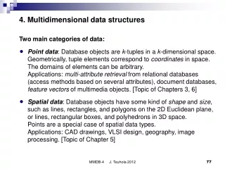
Multidimensional Data • Many applications of databases are ``geographic'' = 2dimensional data. Others involve large numbers of dimensions. • Example: data mining information about sales. • A sale is described by (store, day, item, color, size, etc.). Sale = point in 5dim space. • A customer is described by (age, salary, pcode, maritalstatus, etc.). Typical Queries • Range queries: ``How many customers for gold jewelry have age between 45 and 55, and salary less than 100K?'' • Nearest neighbor : ``If I am at coordinates (x,y), what is the nearest McDonalds.'' • They are expressible in SQL. Do you see how?
SQL • Range queries: ``How many customers for gold jewelry have age between 45 and 55, and salary less than 100K?'‘ SELECT * FROM Customers WHERE age>=45 AND age<=55 AND sal<100; • Nearest neighbor : ``If I am at coordinates (a,b), what is the nearest McDonalds.'‘ Suppose we have a relation Points(x,y,name) SELECT * FROM Points p WHERE p.name=‘McDonalds’ AND NOT EXISTS ( SELECT * FROM POINTS q WHERE (q.x-a)*(q.x-a)+(q.y-b)*(q.y-b) < (p.x-a)*(p.x-a)+(p.y-b)*(p.y-b) AND q.name=‘McDonalds’ );
Big Impediment • For these types of queries, there is no clean way to eliminate lots of records that don't meet the condition of the WHEREclause. Approaches • Index on attributes independently. • Intersect pointers in main memory to save disk I/O. • Problem: Does this structure help with the nearestneighbor? • Multiple key index: Index on one attribute provides pointer to an index on the other.
Computing aggregates • Sales(day,store,item,color,size) • Such relations are called “Data cube” • Example query: • “Summarize the sales of white shirts by day and store.” SELECT FROM Sales s WHERE s.item=‘Shirt’ AND s.color=‘white’ GROUP BY day, store;
Attempt at using B-trees for MD-queries • Database = 1,000,000 points evenly distributed in a 1000×1000 square. Stored in 10,000 blocks (100 recs per block) • Range query {(x,y) : 450 x 550, 450 y 550} • B-tree indexes with pointer lists on x and on y • 100,000 pointers (i.e. 1,000,000/10) for x, and same for y • 10,000 pointers for answer (found by pointer intersection) • Root of each B-tree in main memory • Suppose leaves have avg. 200 keys 500 disk I/O in each B-tree to get pointer lists 1000 + 2(for intermediate B-tree level) disk I/O’s • Retrieve 10,000 records. If they are stored randomly we need to do 10,000 I/O’s • Sum 11,002 disk I/O’s • Sequential scan of file = 10,000 I/O’s (100 tuples per block)
Nearest Neighbor query using B-trees • Turn NN to (10,20) into a range-query {(x,y):10-d x 10+d, 20-d y 20+d } • Possible problem: • No point in the selected range • The closest point inside may not be the answer • Solution: re-execute range query with slightly larger d
NN-queries, example • Same relation Points and its indexes on x and y as before, and Query: NN to (10,20) • Choose d = 1 range-query = {(x,y): 9x 11, 19y21} • 2000 points in [9,11], same in [19,21] each dimension = 10+1 I/O’s to get pointers (+1 is because points with x=9 may not start just at the beginning of the leaf) • With an extra I/O for the intermediate node for each index 24 + 1 disk I/O’s to get the answer, assuming 1 of the 4 points is the answer, which we can determine by their coordinates, prior to getting the data blocks holding the points • However, if d is too small, we have to run another range query with a larger d
Grid files (hash-like structure) • Divide data into stripes in each dimension • Rectangle in grid points to bucket • Example: database records (age,salary) for people who buy gold jewelry. Data: (25,60) (45,60) (50,75) (50,100) (50,120) (70,110) (85,140) (30,260) (25,400) (45,350) (50,275) (60,260)
Operations Lookup Find coordinates of point in each dimension --- gives you a bucket to search. Nearest Neighbor Lookup point P . Consider points in that bucket. • Problem: there could be points in adjacent buckets that are closer. • Example: NN of (45; 200). • Problem: there could be no points at all in the bucket: widen search? Range Queries Ranges define a region of buckets. • Buckets on border may contain points not in range. • Example: 35 < age <= 45; 50 < salary <= 100. Queries Specifying Only One Attribute • Problem: must search a whole row or column of buckets.
Insertion • Use overflow buckets, or split stripes in one or more dimensions • Insert (52,200). Split central bucket, for instance by splitting central salary stripe • The blocks of 3 buckets are to be processed. • In general the blocks of n buckets are to be processed during a split. • n is the number of buckets in the chosen direction • Very expensive.
Insertion • Insert (52,200). Split central bucket, for instance by splitting central salary stripe (One possibility)
Grid files Advantages • Good for multiple-key search • Supports PM, RQ, NN queries Disadvantages • Space, management overhead • Need partitioning ranges that evenly split keys • Possibility of overflow buckets for insertion
Partitioned hashing I • If we hash the concatenation of several keys then such a hash table cannot be used in queries specifying only one dimension (key). • A preferable option is to design the hash function so it produces some number of bits, say k. These k bits are divided among n attributes. • I.e. the hash function h is a concatenation of n hash functions, one for each dimensional attribute. • h = (h1, …, hn) • the bucket where to put a tuple (v1, …, vn) is computed by concatenating the bit sequences h1(v1)…hn(vn).
Partitioned hashing II • If we have a hash table with 10-bit bucket numbers (1024 buckets), we could devote four bits to attribute a and the remaining six bits to attribute b. • We hash using ha and hb. • If we are given a partial match query specifying only the value of a, we compute ha(a), which could be, say 0101. Then, we locate all the relevant buckets, which are: 0101000000 to 0101111111.
Partitioned hashing III • Example: Gold jewelry with • first bit = age mod 2 • bits 2 and 3: salary mod 4 • Works well for: • partial match (i.e. just an attribute specified) • Bad for: • range • Nearest Neighbors queries
Grid files vs. partitioned hashing • If many dimensions many empty cells in grid. While partitioned hashing is OK. • Both support exact and partial match queries. • Grid files good for range and Nearest Neighbor queries, while partitioned hashing is not at all.