Multidimensional R-Trees & Bitmap Indexes
Discover how R-trees support queries and insertion for multidimensional data, and how Bitmap Indexes optimize data retrieval through bitmaps. Learn about basic compression techniques in database management. Explore the power and efficiency of indexing methods.

Multidimensional R-Trees & Bitmap Indexes
E N D
Presentation Transcript
Multidimensional Data Rtrees Bitmap indexes
R-Trees • For “regions” (typically rectangles) but can represent points. • Supports NN, “whereamI” queries. • Generalizes Btree to multidimensional case. • In place of Btree's keypointer pairs, Rtree has regionpointer pairs.
Lookup – Where Am I? • We start at the root, with which the entire region is associated. • We examine the subregions at the root and determine which children correspond to interior regions that may contain point P. • If there are zero regions we are done; P is not in any data region. • If there are some subregions we must recursively search those children as well, until we reach the leaves of the tree.
Insertion Inserting region R. 1. We start at the root and try to find some subregion into which R fits. • If more than one we pick just one, and repeat the process there. 2. If there is no region, we expand, and we want to expand as little as possible. • So, we pick the child that will be expanded as little as possible. 3. Eventually we reach a leaf, where we insert region R. 4. However, if there is no room we have to split the leaf. • We split the leaf in such a way as to have the “smallest subregions.”
Example • Suppose that the leaves have room for six regions. • Further suppose that the six regions are together on one leaf, whose region is represented by the outer solid rectangle. • Now suppose that another region POP is added.
Example (Cont’ ed) ((0,0),(60,50)) ((20,20),(100,80)) Road1 Road2 House1 School House2 Pipeline Pop
Example (Cont’ ed) • Suppose now that House3 ((70,5),(80,15)) gets added. • We do have space in the leaves, but we need to expand one of the regions at the parent. • We choose to expand the one which needs to be expanded the least.
We chose this option because it produces the smallest increase in total surface area Which one should we expand? ((0,0),(80,50)) ((20,20),(100,80)) Road1 Road2 House1 House3 School House2 Pipeline Pop Two choices: ((0,0),(60,50)) ((20,5),(100,80)) Road1 Road2 House1 School House2 Pipeline Pop House3
Bitmap Indexes • Suppose we have n tuples. • A bitmap index for a field F is a collection of bit vectors of length n, one for each possible value that may appear in the field F. • The vector for value v has 1 in position i if the i-th record has v in field F, and it has 0 there if not. (30, foo) (30, bar) (40, baz) (50, foo) (40, bar) (30, baz) foo 100100 bar 0… baz …
Graphical Picture Customer table. We will index Gender and Rating. Note that this is just a partial list of all the records in the table Two bit strings for the Gender bitmap Five bit strings for the Rating bitmap
Bitmap operations • Bit maps are designed to support partial match and range queries. How? • To identify the records holding a subset of the values from a given dimension, we can do a binary OR on the bitmaps from that dimension. • For example, the OR of bit strings for Age = (20, 21, 22) • To identify the partial matches on a group of dimensions, we can simply perform a binary AND on the OR-ed maps from each dimension. • These operations can be done very quickly since binary operations are natively supported by the CPU.
1 0 1 1 0 1 1 1 OR = 0 1 1 1 1 1 0 0 1 1 0 0 0 0 1 1 1 1 AND = 0 First two records in our fact table are retrieved 0 Bit Map example SELECT * FROM Customer WHERE gender = M AND (rating = 3 OR rating = 5)
Gold-Jewelry Data (25; 60) (45; 60) (50; 75) (50; 100) (50; 120) (70; 110) (85; 140) (30; 260) (25; 400) (45; 350) (50; 275) (60; 260) What would be the bitmap index for age, and the bitmap index for salary? • Suppose we want to find the jewelry buyers with an age in the range 45-55 and a salary in the range 100-200. What do we do?
How big do these things get? • Assuming each attribute value fits in a 32-bit machine word, the bitmap index for an attribute with value cardinality 32 takes as much space as the base data column. • Since a B-tree index for a 32-bit attribute is often observed to use 3 or 4 times the space as the base data column, many users consider attributes with cardinalities less than 100 to be suitable for using bitmap indices. • However, some other users believe bit map indexes are good for attributes with cardinalities more than 100. What can be done?
Basic Compression • Run length encoding is used to encode sequences or runs of zeros. • Say that we have 20 zeros, then a 1, then 30 more zeros, then another 1. • Naively, we could encode this as the integer pair <20, 30> • This would work. But what's the problem? • On a typical 32-bit machine, an integer uses 32 bits of storage. So our <20, 30> pair uses 64 bits. The original string only had 52!
Basic Compression (Cont'd) • So we must use a technique that stores our run-lengths as compactly as possible. • Let’s say we have the string 000101 • This is made up of runs with 3 zeros and 1 zero. • In binary, 3 = 11, while 1 is, of course, just 1 • This gives us a compressed representation of 111. • The problem? • How do we decompress this? • We could interpret this as 1-11 or 11-1 or even 1-1-1. • This would give us three different strings after the decompression.
Example: 000000000000010000001 • Here we have two “0” runs of length 13 and 6 • 13 can be represented by 4 bits, 6 requires 3 bits • Run 1: j – 1 “1” bits + 0 + i → 111 0 1101 • Run 2: j – 1 “1” bits + 0 + i → 11 0 110 • Final compressed string: 11101101110110 • Compression rate: (21-14)/21 = 33% Proper RLE encoding • Run of length i has i 0’s followed by a 1. • Let’s say that that we have a run of length i. • Let j be the number of bits required to represent i. • To define a run, we will use two values: • The “unary” representation of j • A sequence of j – 1 “1” bits followed by a zero (the zero signifies the end of the unary string) • The special cases of j = 0 and j = 1 use 00 and 01 respectively. • The value i (using j bits)
Decoding • Let’s decode 11101101001011 11101101001011 13 11101101001011 0 11101101001011 3 Our sequence of run lengths is: 13, 0, 3. What’s the bitmap? 0000000000000110001
Summary Pros: • Bitmaps provide efficient storage for low cardinality dimensions. On sparse, high cardinality dimensions, compression can be effective. • Bit operations can support multi-dimensional partial match and range queries Cons: • De-compression requires run-time overhead • Bit operations on large maps and with large dimension counts can be expensive.