Download
1 / 51
510 likes | 617 Views
The Critical Role of Primary Occurrence Data in Biodiversity Modeling Keeping Data and Products Alive. A. Townsend Peterson Natural History Museum The University of Kansas. Keeping Biodiversity Information Alive I. Biodiversity information exists in two forms:

E N D
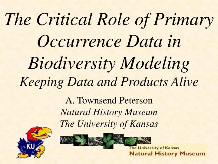
The Critical Role of Primary Occurrence Data in Biodiversity ModelingKeeping Data and Products Alive A. Townsend Peterson Natural History Museum The University of Kansas
Keeping Biodiversity Information Alive I • Biodiversity information exists in two forms: • primary data - specimens and observations, studies of the organism, etc. • secondary information - summaries, range maps, field guides, county records
Secondary Information Primary data
Keeping Biodiversity Information Alive II • Basing analyses and prioritizations on secondary products is convenient, but ...
Keeping Biodiversity Information Alive II • Basing analyses and prioritizations on secondary products is convenient, but ... • Severs the vital connection between product and data - product begins to degrade
Data and Product Degradation The statement is made ... “Species X is present at Site Y” Almost immediately, new information becomes available, taxonomies are redone, landscapes and patterns of land use change, and data become less meaningful. Hence, data quality and meaning, as well as quality and meaning of products based on the data, begin to degrade.
Keeping Biodiversity Information Alive II • Basing analyses and prioritizations on secondary products is convenient, but ... • Severs the vital connection between product and data - product begins to degrade • Does not allow product to grow, improve, and evolve with more and better data
Product Evolution and Improvement • Most biodiversity data sets grow by 1-5% yearly... data (and products based on the data) get better through time • More data sets are computerized and should be available each year • Improvement in technology and data availability for land-use evaluation permits better contextual understanding
Keeping Biodiversity Information Alive II • Basing analyses and prioritizations on secondary products is convenient, but ... • Severs the vital connection between product and data - product begins to degrade • Does not allow product to grow, improve, and evolve with more and better data • Loses opportunity to take advantage of new, quantitative approaches for distributional modeling and synthetic analysis
Keeping Biodiversity Information Alive III • Using primary information, especially point occurrence data, solves many problems: • Applicable to all regions and all taxa • Products don’t get old; rather, they update and evolve with improved information - product gets better • Products not limited to original planned purpose for which they were developed
Keeping Biodiversity Information Alive IV • Primary point occurrence data offer several distinct advantages... • Species’ occurrences are referenced to particular points in space, permitting characterization of ecological needs • Species’ occurrences are referenced to particular points in time, permitting evaluation of temporal changes • Point occurrence data lend themselves well to statistical and other quantitative approaches • Products can be developed at any scale, from meters to continents • Products are verifiable, making quality assessment possible • No subjective, intermediate interpretive steps involved
Mexican Bird Collections British Museum Paris Field Museum KU Natural History Museum
Example North American DataThe U.S. Breeding Bird Survey(soon to be added to the Species Analyst!)
New Facility for Sharing Biodiversity Data .... The Species Analyst North American Biodiversity Information Network A distributed database for biodiversity information, linking institutions and serving data to all potential users http://chipotle.nhm.ukans.edu/nabin/
The Challenge of Inferring Geographic Distributions 4. Inference beyond the limits of the actual data becomes necessary 1. Existing sampling is incomplete 2. Gaps in known distribution can represent real absence or simply nondetection 3. Without more data distinguishing between these two possibilities is not possible
Two Types of Error in Distributional Predictions Actual geographic distribution
Two Types of Error in Distributional Predictions Predicted geographic distribution
Two Types of Error in Distributional Predictions Actual geographic distribution Predicted geographic distribution
Two Types of Error in Distributional Predictions Actual geographic distribution Predicted geographic distribution Overprediction, or Commission Underprediction, or Omission
Two Types of Error in Distributional Predictions Objective: To Minimize Both Forms of Error
Two Types of Error in Distributional Predictions Objective: To Minimize Both Forms of Error
Predictive Methodologies I • Georeferenced occurrence points • Electronic maps ... geographic coverages ... summarizing environmental dimensions important to species, such as temperature, rainfall, topography, soils, geology, etc. • Use nonrandom associations between points and coverages to build a model of a species’ ecological niche • Project model back onto geography to predict distribution
Predictive Methodologies II • Subset points into a training dataset (for building models) and a test dataset (for assessing their effectiveness • Apply an algorithm to training data • BIOCLIM • logistic regression • discriminant function analysis • distance measures • etc. • Assess effectiveness of model, asking whether observed omission and commission are significantly less than random
BIOCLIM Example Occurrence points overlain on geographic coverage, such as rainfall
BIOCLIM Example Occurrence points overlain on geographic coverage, such as rainfall Frequency histogram of occurrence points in rainfall classes
BIOCLIM Example Occurrence points overlain on geographic coverage, such as rainfall Frequency histogram of occurrence points in rainfall classes Distribution trimmed to eliminate marginal habitat records
BIOCLIM Example Occurrence points overlain on geographic coverage, such as rainfall Frequency histogram of occurrence points in rainfall classes Distribution trimmed to eliminate marginal habitat records Project trimmed distribution
Genetic Algorithm for Rule-set Prediction(GARP) • Developed by David Stockwell, San Diego Supercomputer Center • Takes advantage of multiple algorithms (BIOCLIM, logistic regression, etc.) • Different decision rules may apply to different sectors of species’ distributions • Uses a genetic algorithm, an artificial intelligence application, for choosing rules • Implemented on WWW, and open for public use (http://biodi.sdsc.edu)
Example of Heterogeneous Rule Sets in GARP TRANSLATE - model into natural language No-rule number, Type, Prior-prior, Post-accuracy, Sig-Significance, Cov-coverage, Use-usage No Type Prior Post Sig Cov Use 1 m 0.50 0.92 26.66 0.41 0.376; IF Veg=[ 0, 9]r AND Elev=[ 0,2233]r AND Precip=[ 0, 9]r AND Temp=[ 0, 2]r AND Latitude=[25.1,15.2]r AND Longitud=[-107.6,-93.0]r AND Coastal=[0.0,131.0]r THEN Taxon=PRESENT 8 r 0.48 1.00 21.32 0.17 0.166; IF + Veg*0.02 r + Precip*0.29 r - Temp*0.26 r - Latitude*0.45 r + Longitud*0.27 r - Coastal*0.43 r THEN Taxon=BACKGROUND 0 r 0.51 0.98 27.10 0.32 0.127; IF - Veg*0.25 r + Elev*0.12 r + Precip*0.32 r + Temp*0.45 r - Latitude*0.43 r + Longitud*0.18 r - Coastal*0.50 r THEN Taxon=BACKGROUND 6 r 0.49 0.81 23.16 0.51 0.071; IF + Veg*0.38 r - Elev*0.49 r + Precip*0.02 r - Temp*0.36 r + Latitude*0.16 r - Longitud*0.21 r - Coastal*0.30 r THEN Taxon=PRESENT 14 d 0.51 0.85 19.33 0.32 0.066; IF Elev=[99,1245]r AND Precip=[ 3, 5]r AND Temp=[ 0, 3]r THEN Taxon=PRESENT 2 r 0.48 0.92 26.52 0.36 0.060; IF + Veg*0.02 r + Elev*0.49 r + Precip*0.17 r + Temp*0.17 r - Latitude*0.36 r - Longitud*0.02 r - Coastal*0.50 r THEN Taxon=BACKGROUND 3 r 0.48 0.89 25.83 0.39 0.040; IF - Veg*0.43 r + Elev*0.11 r - Precip*0.02 r + Temp*0.34 r - Latitude*0.02 r + Longitud*0.19 r - Coastal*0.50 r THEN Taxon=BACKGROUND 13 d 0.49 1.00 19.36 0.15 0.038; IF Elev=[336,2233]r AND Precip=[ 7, 7]r AND Temp=[ 0, 5]r AND Latitude=[30.0,18.7]r THEN Taxon=BACKGROUND 4 r 0.50 0.91 24.57 0.36 0.029; IF - Veg*0.32 r + Elev*0.07 r + Precip*0.47 r - Temp*0.39 r - Latitude*0.39 r + Longitud*0.50 r - Coastal*0.50 r THEN Taxon=BACKGROUND
GARP Comparison of GARP and BIOCLIM Example: Aratinga canicularis Note extreme over- prediction (commission) in BIOCLIM map BIOCLIM
How Well Can We Predict? • Numerous preliminary efforts showed promise ... good balance between omission and commission • 25 species chosen randomly from the Mexican avifauna for testing • Ability to predict into areas not included in the training data set taken as a measure of model quality • Each species tested in Oaxaca and Jalisco with Lisa Ball and Kevin Cohoon
How Well Can We Predict? Atlapetes pileatus all known occurrence points in Mexico with Lisa Ball and Kevin Cohoon
Removing Points from Test State State of Jalisco with Lisa Ball and Kevin Cohoon
Distributional Model for Points with Lisa Ball and Kevin Cohoon
Focus on Prediction for Test State with Lisa Ball and Kevin Cohoon
Overlay Test Points with Lisa Ball and Kevin Cohoon
How Well Can We Predict? Answer: Reasonably well ... about 85-90% of the species with Lisa Ball and Kevin Cohoon
How Well Can We Predict? Choose training and test states
How Well Can We Predict? Plot training points - Toxostoma rufum
How Well Can We Predict? Develop GARP model
How Well Can We Predict? Overlay test data points
How Well Can We Predict? 715 of 741 test points correctly predicted 34% of total area predicted present 252 points expected to be predicted at random Statistical significance P< 10-225 All 34 species tested significant, no probability exceeding 10-3
Advantages Over Range Maps • Smaller predictions, much greater precision • Reduces errors of commission, which are especially critical • Comparisons in Mexico indicate 103 - 1022 times more statistically significant than range maps • Models improve over time, rather than degrading continually from time of publication • Not limited to areas with published range maps • Produces ecological model (wait a minute...)
Predicting Geographic Distributions Makes Possible ... • Understanding rare and endangered species’ distributions • Designing reintroduction programs • Understanding the effects of global climate change and other types of change • Projecting species invasions • Designing biodiversity conservation plans
Building Maps of Species Diversity Reserve Locations in Southwestern Mexican Dry Forest Primary concentration of endemic species (12) Secondary concentration (4 species) with Daniel A. Kluza
Invasive Species and Endangered Species Barred Owls invading the range of Spotted Owls
Predicting the Effects of Global Climate Change Ortalis poliocephala Before (green) vs. After (red)
Primary Point Occurrence Data • Offer many advantages over secondary information • Applicable across spatial scales, verifiable • Open doors to new, synthetic analyses • Abundantly available for most taxa in most regions • Integrated with new data-sharing efforts • Primary point occurrence data form the most appropriate basis for gap analysis applications