UNIT 15 Query Optimization
UNIT 15 Query Optimization. Contents. 15.1 Introduction to Query Optimization 15.2 The Optimization Process: An Overview 15.3 Optimization in System R 1 5 . 4 Optimization in INGRES 1 5 . 5 Implementing the Join Operators. 15.1 Introduction to Query Optimization. The Problem.

UNIT 15 Query Optimization
E N D
Presentation Transcript
Contents • 15.1 Introduction to Query Optimization • 15.2 The Optimization Process: An Overview • 15.3 Optimization in System R • 15.4 Optimization in INGRES • 15.5 Implementing the Join Operators
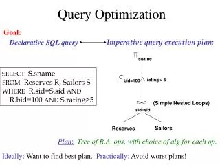
The Problem • How to choose an efficient strategy for evaluating a given expression (a query). • Expression (a query): e.g. select distinct S.SNAME from S, SP where S.S# =SP.S# and SP.P#= 'p2' • Evaluate: • Efficient strategy: • First class e.g. (A join B) where condition-on-B (A join (B where condition-on-B) ) e.g. SP.P# = 'p2' • Second class e.g. from S, SP ==> S join SP How to implement join operation efficiently? • “Improvement" may not be an "optimal" version. §15.5 Implementing the Join Operators
Language Processor Language Processor Optimizer • ? Operator Processor Access Method Access Method File System database Query Processing in the DBMS Query in SQL: SELECT CUSTOMER. NAME FROM CUSTOMER, INVOICE WHERE REGION = 'N.Y.' AND AMOUNT > 10000 AND CUTOMER.C#=INVOICE.C# Internal Form : P(σ(S SP) Operator : SCAN C using region index, create C SCAN I using amount index, create I SORT C?and I?on C# JOIN C?and I?on C# EXTRACT name field Calls to Access Method: OPEN SCAN on C with region index GET next tuple . . . Calls to file system: GET10th to 25th bytes from block #6 of file #5
S SP STATUS CITY S# SNAME P# S# QTY . . . . . . . . . . . . 1 2 . 100 S2 . . . . . . . . S3 S1 . S2 1 2 . 10,000 S5 . S1 An Example Suppose: |S| = 100, |SP| = 10,000, and there are 50 tuples in SP with p# = 'p2'? Results are placed in Main Memory. Query in SQL: SELECT S.* FROM S,SP WHERE S.S# = SP.S# AND SP.P# = 'p2‘ • Method 1: iteration (Join + Restrict) Cost = 100 * 10,000 = 1,000,000 tuple I/O's
SP SP' P# S# QTY P# S# QTY . . . . . . . . S3 S1 . S2 P4 P2 . P2 1 2 . 10000 S1 S3 . S2 P2 P2 . P2 1 2 . 50 An Example (cont.) • Method 2: Restriction iteration Join restrict p#= 'p2' S SP' P# STATUS CITY S# QTY S# SNAME . . . . . . . . . . . . S1 S3 . S2 . . . . 1 2 . 50 P2 P2 . P2 1 2 . 100 S2 S5 . S1 cost = 10,000 + 100 * 50 = 15,000 I/O
An Example (cont.) • Method 3: Sort-Merge Join + Restrict Suppose S, SP are sorted on S#. S SP S# P# QTY S1 S1 . . . S100 S# SNAME STATUS CITY S1 S2 . . . S100 1 2 . . . 10,000 . . . . 1 2 . . . 100 . . . . . . . . . . . . . . . . cost = 100 + 10,000 = 10,100 I/O
15.2 The Optimization Process: An Overview (1) Query => internal form (2) Internal form => efficient form (3) Choose candidate low-level procedures (4) Generate query plans and choose the cheapest one
Algebra: ( (S join SP) where P#= 'P2') [SNAME] or ( ( S SP) ) SNAME 'P2' S.S# = SP.S# Query => Algebra Step 1: Cast the query into some internal representation Query: "get names of suppliers who supply part p2" SQL:select distinct S.SNAME from S,SP where S.S# = SP.S# and SP.P# = 'p2' Query tree: result | project (SNAME) | restrict (SP.P# = 'p2') | join (S.S# = SP.S#) S SP
C Step 2: Convert to equivalent and efficient form • Def: Canonical Form Given a set Q of queries, for q1, q2 belong to Q, q1 are equivalent to q2 (q1 q2) iff they produce the same result, Subset C of Q is said to be a set of canonical forms for Q iff • Note: Sufficient to study the small set C • Transformation Rules Q Step2 • output of step1 trans. equivalent and more • efficient form Algebra Efficient Algebra
C Step 2: Convert to equivalent and efficient form (cont.) e.g.1 [restriction first] (A join B) where restriction_B A join ( B where restriction_B) e.g.2 [More general case] (A join B) where restriction_A and restriction_B (A where rest_on_A) join ( B where rest_on_B) e.g.3 [ Combine restriction] ( A where rest_1 ) where rest_2 A where rest_1 and rest_2 q1 q1≡q2 q2 scan 2 1
n1<n n+n1 Step 2: Convert to equivalent and efficient form (cont.) e.g.4 [projection] last attribute (A [attribute_list_1] ) [attri_2] A [attri_2] e.g.5 [restriction first] (A [attri_1]) where rest_1 (A where rest _1) [attri_1] . . . .
SP P P# S# P# QTY P1 P2 P3 P4 P5 S1 S2 Step 2: Convert to equivalent and efficient form (cont.) e.g.6 [Introduce extra restriction] SP JOIN (P WHERE P.P#= 'P2') (SP WHERE SP.P# = 'P2') JOIN (P WHERE P.P# = 'P2') e.g.7 [Semantic transformation] (SP join P ) [S#] SP[S#] Note: a very significant improvement. Ref.[17.27] P.571 J. J. King, VLDB81 sp.p# = p.p# if restriction on join attribute sp.p# = p.p# if SP.P# is a foreign key matching the primary term P.P#
Step 3: Choose candidate low-level procedures • Low-level procedure • e.g. Join, restriction are low-level operators • there will be a set of procedures for implementing each operator, e.g. Join (ref p.11-31) <1> Nested Loop (a brute force) <2> Index lookup (if one relation is indexed on join attribute) <3> Hash lookup (if one relation is hashed by join attribute) <4> Merge (if both relations are indexed on join attribute) . . .
( (C I)) 6 choose 2 Step 3: Choose candidate low-level procedures (cont.) SQL Algebra • Data flow Canonical Form e.g. System catalog existence of indexes cardinalities of relations Optimizer step3 : access path selection . . . . Lib predefined low-level procedures Ref. p.11-31 p.554 One or more candidate procedures for each operator e.g. , , 2 3 2 Step4
Step 4: Generate query plans and choose the cheapest • Query plan • is built by combing together a set of candidate implementation procedures • for any given query many many reasonable plans Note: may not be a good idea to generate all possible plans. heuristic technique "keep the set within bound" (reducing the search space)
Step 4(a) ( (C I)) query plans Step 4(b) choose the cheapest 2 2 1 cheapest Step 4: Generate query plans and choose the cheapest (cont.) • Data flow output of step 3 2 3 2 ... 1 2 1
Step 4: Generate query plans and choose the cheapest (cont.) • Choosing the cheapest • require a method for assigning a cost to any given plan. • factor of cost formula: (1) # of disk I/O (2) CPU utilization (3) size of intermediate results • a difficult problem [Jarke 84, 17.3. p.564 ACM computing surveys] [Yao 79, 17.8 TODS] . . .
Optimization in System R • Only minor changes to DB2 and SQL/DS. • Query in System R (SQL) is a set of "select-from-where" block • System R optimizer step1: choosing block order first in case of nested => innermost block first step2: optimizing individual blocks Note: certain possible query plan will never be considered. • The statistical information for optimizer Where: from the system catalog What: 1. # of tuples on each relation 2. # of pages occupied by each relation. 3. percentage of pages occupied by each relation. 4. # of distinct data values for each index. 5. # of pages occupied by each index. . . . Note: not updated every time the database is updated. (overhead??)
Optimization in System R (cont.) • Given a query block • case 1. involves just a restriction and/or projection • 1. statistical information (in catalog) • 2. formulas for size estimates of intermediate results. • 3. formulas for cost of low-level operations (next section) • choose a strategy for constructing the query operation. • case 2. involves one or more join operations • e.g. A join B join C join D • ((A join B) join C) join D • Never: (A join B) join (C join D) Why? See next page
Note: 1. "reducing the search space" 2. heuristics for choosing the sequence of joins are given in [17.34] P.573 3. (A join B) join C not necessary to compute entirely before join C i.e. if any tuple has been produced It may never be necessary to finish relation "A B ", why ? pass to join C Optimization in System R (cont.) • ((A join B) join C) join D • Never: (A join B) join (C join D) ∵ C has run out ??
Optimization in System R (cont.) • How to determine the order of join in System R ? • consider only sequential execution of multiple join. <e.g.> ((A B) C) D (A B) (C D) × STEP1: Generate all possible sequences <e.g.> (1) ((A B) C) D (2) ((A B) D) C (3) ((A C) B) D (4) ((A C) D) B (5) ((A D) B) C (6) ((A D) C) B (7) ((B C) A) D (8) ((B C ) D) A (9) ((B D) A) C (10) ((B D) C) A (11) ((C D) A) B (12) ((C D) B) A Total # of sequences = ( 4! )/ 2 = 12
Optimization in System R (cont.) STEP 2: Eliminate those sequences that involve Cartesian Product • if A and B have no attribute names in common, then A B = A x B STEP 3: For the remainder, estimate the cost and choose a cheapest.
detach P Query Decomposition • a general idea for processing queries in INGRES. • basic idea: break a query involving multiple tuple variables down into a sequence of smaller queries involving one such variable each, using detachment and tuple substitution. • avoid to build Cartesian Product. • keep the # of tuple to be scanned to a minimum. <e.g> "Get names of London suppliers who supply some red part weighing less than 25 pounds in a quantity greater than 200" Initial query: Q0: RETRIEVE (S.SNAME) WHERE S.CITY= 'London' AND S.S# = SP.S# AND SP.QTY > 200 AND SP.P# = P.P# AND P.COLOR = Red AND P.WEIGHT < 2 5
detach SP detach S Query Decomposition (cont.) D1: RETRIEVE INTO P' (P.P#) WHERE P.COLOR= 'Red' AND P.WEIGHT < 25 Q1: RETRIVE (S.SNAME) WHERE S.CITY = 'London' AND S.S# = SP.S# AND SP.QTY > 200 AND SP.P# = P'.P# S join SP join P’ D2: RETRIEVE INTO SP' (SP.S#, SP.P#) WHERE SP.QTY > 200 Q2: RETRIEVE (S.SNAME) WHERE S.CITY = 'London' AND S.S#=SP'.S# AND SP'.P#=P'.P#
Query Decomposition (cont.) D3: RETRIEVE INTO S' (S.S#, S.SNAME) WHERE S.CITY = 'LONDON' Q3: RETRIEVE (S'.SNAME) WHERE S'.S# =SP'.S# AND SP'.P# = P'.P# D4: RETRIEVE INTO SP"(SP'.S#) WHERE SP'.P# =P'.P# Q4: RETRIEVE (S'.SNAME) WHERE S'.S# = SP".S# D5: RETRIEVE INTO SP"(SP'.S#) WHERE SP'.P# = 'P1' OR SP'.P#= 'P3‘ Q5: RETRIEVE (S'.SNAME) WHERE S'.S# = 'S1' OR S'.S# = 'S2' OR S'.S# = 'S4' detach P' and SP' D4: two var. --> tuple substitution ( Suppose D1 evaluate to {P1, P3 } Q4 : two var. --> tuple substitution ( Suppose D5 evaluate to { S1, S2, S4})
Query Decomposition (cont.) • Decomposition tree for query Q0: • D1, D2, D3: queries involve only one variable => evaluate • D4, Q4: queries involve tow variable => tuple substitution • Objectives : • avoid to build Cartesian Product. • keep the # of tuple to be scanned to a minimum. Overall result Q4 (Q5) SP'' S' D4 (D5) D3 SP' P' D2 D1 S SP P
15.5 Implementing the Join Operators Method 1: Nested Loop Method 2: Index Lookup Method 3: Hash Lookup Method 4: Merge
R S . . . . . . . . . . . . . . . . . . . . A A . . . . . . . . . . . . . . . . . . . . 1 a b 1 b a . . e . . a m n Join Operation • Suppose R S is required, R.A and S.A are join attributes.
. . . . . . . . . . . . . . . . . . . . A A . . . . . . . . . . . . . . . . . . . . 1 b a 1 a b . . a . . e n m Method 1: Nested Loop • Suppose R and S are not sorted on A. R S • O (mn) • the worst case • assume that S is neither indexed nor hashed on A • will usually be improved by constructing index or hash on S.A dynamically and then proceeding with an index or hash lookup scan.
. . . . A . . . . . . . . . . . . . . . . b a . . a Method 2: Index Lookup • Suppose S in indexed on A S S.A_index R . . . . . . . . . . A a . . . . . 1 n . . . . . a 1 a b . . e . . . . b m . . . .
S . . . . . . . . . . R S.A . . . . . . . . . . R.A . . . . b . . . . . . 0 1 2 h(a) . . . . . . . . . . . . . . . . . . . . . . . . .. . . . . . . . . 1 a b z e a . . . . . e m h(e) . . . z . . h(e) = 1 h(b) = 0 h(a) = 2 h(z) = 2 . . . a . . Method 3: Hash Lookup • Suppose S is hashed on A. • Calculate hash function is faster than search in index.
R . . . . . . . . . . A . . . . . . . . . . a b 1 n 1 S b c z . . . . . . . . . . A . . . . . . . . . . a a m b b d S R . . . . . . . . . . . . . . . . . . . . a A a A . . . . . . . . . . b a a . . . . . . . . . . b a a b d b a z c b = Method 4: Merge • Suppose R and S are both sorted (for indexed) on A. • Only index is retrieved for any unmatched tuple.


