Download
1 / 343
3.43k likes | 3.54k Views
Understand linear systems of equations, vectors, vector addition, and linear transformations. Explore applications in NumPy and geometric interpretations. Learn about homogeneous systems, linear independence, and key principles in linear algebraic operations.

E N D
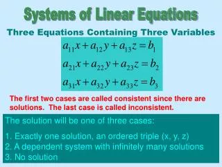
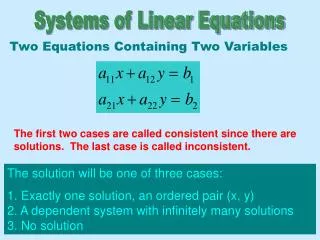
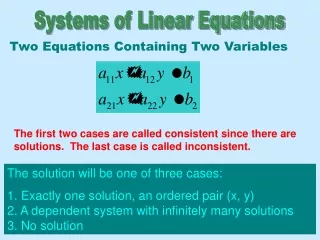
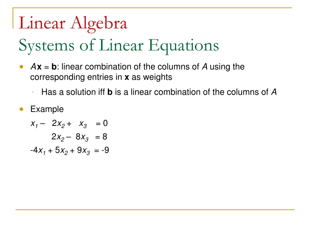
Linear AlgebraSystems of Linear Equations • Ax = b: linear combination of the columns of A using the corresponding entries in x as weights • Has a solution iff b is a linear combination of the columns of A • Example x1 – 2x2 + x3 = 0 2x2 – 8x3 = 8 -4x1+ 5x2 + 9x3 = -9
>>> from numpy import * >>> A = array([[1,-2,1], [0,2,-8], [-4,5,9]]) >>> b = array([0,8,-9]) >>> from numpy.linalg import * >>> x = solve(A, b) >>> print x [ 29. 16. 3.] >>> dot(A[0], x) 0.0 >>> dot(A[1], x) 8.0 >>> dot(A[2], x) -9.0 >>> dot (A, x) array([ 0., 8., -9.])
Vectors in Rn • Given a vector u and a real number c, the scalar multiple of u by c is the vector cu got by multiplying each entry in u by c >>> print 1.2 * array([2,3]) [ 2.4 3.6] Geometric interpretation of vectors (R2) • Each point in the plane is determined by a pair of numbers • Identify a geometric point (a, b) with the column vector [ab]T Parallelogram Rule for Addition • For u and v in R2, u + v corresponds to the 4th vertex of the parallelogram whose other vertices are u, 0, and v
>>> print array([2,2]) + array([-6,1]) [-4 3] • The 0 vector contains all 0’s and is the identity element for vector addition >>> print array([1,2]) + zeros(2) [ 1. 2.] • Given vectors v1, v2, …, vp in Rn and scalars c1, c2, …, cp, the vector y = c1v1+ c2v2 + … + cpvp is a linear combination of v1, …, vp using weightsc1, …, cp
The Equation Ax = b • Given an mn matrix A with columns a1, …, an and b in Rn, matrix equation Ax = b has the same solution set as the vector equation x1a1+ x2a2+ … + xnan = b • If A is an mn matrix, u and v are vectors in Rn, and c is a scalar, then A(u + v) = Au + Av A(cu) = c(Au)
>>> A = array([[0,1], [1,2]]) >>> u, v = array([1,2]), array([3,1]) >>> print dot(A, u+v) [ 3 10] >>> print dot(A, u) + dot(A, v) [ 3 10] >>> c = 2 >>> print dot(A, c*u) [ 4 10] >>> print c * dot(A, u) [ 4 10]
Vector Addition as Translation • In dynamic terms, vector addition is translation • Given v and p in R2 or R3, the effect of adding p to v is to move v in the direction of p • v is translated byp to v + p
A system of linear equations is homogeneous if it can be written in the form Ax = 0 • It always has at least the trivial solution, x = 0 • Ax = 0 has a nontrivial solution iff the system has at least one free variable • “Free variable”: we are free to chose a value for it • numpy.linalg won’t solve homogeneous systems • The set of vectors {v1, …, vk} in Rn is linearly dependent if there exist weights c1, …, ck s.t. c1v1 + c2v2 + … cknk = 0 • Otherwise, it’s linearly independent
Linear Transformations • The correspondence from x to Ax is a function from one set of vectors to another • A transformation (function or mapping) T from Rn to Rm is a rule that assigns to each vector x in Rn a unique vector T(x) in Rm— • its image under T • Use the usual terms domain and range • For each x in Rn, T(x) is computed as Ax, where A is an mn matrix
Linear transformations preserve the operations of vector addition and scalar multiplication • If T is a linear transformation, then T(0) = 0 T(cu + dv) = cT(u) + dT(v) for all vectors u, v in the domain of T and all scalars c, d • From this, we can derive the superposition principle T(c1v1 + … + cpvp) = c1T(v1) + … + cpT(vp)
Given scalar r, define T: R2R2 by T(x) = rx • A contraction if 0 r 1 • A dilation if r > 1 • T: R2R2 defined by • Rotates CCW through 90 >>> T = array([[0,-1], [1,0]]) >>> print dot(T, array([0.5,0.5])) [-0.5 0.5]
For linear transformation T: RnRm, there exists a unique matrix A s.t. T(x) = Ax for all x in Rn • A is the m n matrix whose j th column is the vector T(ej), where ej is the jth column of the identity matrix in Rm , Im A = [T(e1), …, T(en)] • This is the standard matrix for the linear transformation T • E.g., to find the standard matrix A for the dilation transformation T(x) = 3x, note T(e1) = 3e1 = [3 0]T T(e2) = 3e2 = [0 3]T
NumPy function eye(N) returns an N N identity array (float elements) >>> I2 = eye(2) >>> print I2[:,0], I2[:,1] [ 1. 0.] [ 0. 1.] >>> dil3 = column_stack((3 * I2[:,0], 3 * I2[:,1])) >>> dot(dil3, array([1,2])) array([ 3., 6.])
E.g, Let T: R2R2 rotate points in R2 through angle , CCW for positive angle • [1 0]T rotates into [cos sin ]T • [0 1]T rotates into [- sin cos ]T • So >>> phi = pi/4 >>> cosp, sinp = cos(phi), sin(phi) >>> A = array([[cosp, -sinp], [sinp, cosp]]) >>> print dot(A, array([2,2])) [ 2.22044605e-16 2.82842712e+00]
For the next result, need the following definition If v1, …, vp are vectors in Rn, then the set of all possible linear combinations of v1, …, vp is the subset of Rnspanned by {v1, …, vp} • Let T: RnRm be a linear transformation and A its standard matrix. Then • T maps Rn onto Rm iff the columns of A span Rn • T is one-to-one iff the columns of A are linearly independent
Matrix Operations • Two matrices are compatible for addition iff they have the same size (shape) • Addition is done element-wise >>> arange(4).reshape(2,2) + arange(1,5).reshape(2,2) array([[1, 3], [5, 7]]) >>> arange(4).reshape(2,2) + arange(1,7).reshape(2,3) Traceback (most recent call last): File "<stdin>", line 1, in <module> ValueError: shape mismatch: objects cannot be broadcast to a single shape
If r is a scalar and A a matrix, the scalar multiple rA is the matrix whose columns are r times the corresponding columns of A • As with vectors, -A means (-1)A, A – B means A + (-1)B >>> - arange(4).reshape(2,2) array([[ 0, -1], [-2, -3]]) >>> arange(1,5).reshape(2,2) - arange(4).reshape(2,2) array([[1, 1], [1, 1]]) • The usual rules of algebra apply to sums and scalar multiples of matrices
A(Bx) is produced by a composition of mappings • Represent this composite mapping as multiplication by a single matrix, AB A(Bx) = (AB)x • Matrices A, B are compatible for multiplication iff, for some n, A is mn and B is np • If A is mn and Bnp with columns b1, …, bn, then AB is mp with columns Ab1, …, Abp • Matrix multiplication is not generally commutative • It’s not always true that AB = BA
>>> A = arange(4).reshape(2,2) >>> B = arange(2,10,2).reshape(2,2) >>> print A [[0 1] [2 3]] >>> print B [[2 4] [6 8]] >>> dot(A,B) array([[ 6, 8], [22, 32]]) >>> print array(mat(A) * matrix(B)) [[ 6 8] [22 32]] >>> print dot(B,A) [[ 8 14] [16 30]]
The transpose of mn matrix A, AT, is the nm matrix whose rows are the columns of A >>> A = arange(4).reshape(2,2) >>> print A [[0 1] [2 3]] >>> print A.T [[0 2] [1 3]] >>> print A.transpose() [[0 2] [1 3]] Properties of the Transpose (AT)T = A (A + B)T = AT + BT For scalar r, (rA)T = rAT (AB)T = BTAT
The Inverse of a Matrix • The inverse of nn matrix A, A-1, if it exists, is unique, and AA-1 = I and A-1A = I • If and det A = ad - bc 0, then A is invertible and • If A is an invertible nn matrix, then, for all b in Rn, Ax = b has a unique solution x = A-1b
>>> A = array([[1,-2,1], [0,2,-8], [-4,5,9]]) >>> b = array([0,8,-9]) >>> x = solve(A,b) >>> x array([ 29., 16., 3.]) >>> Ainv = inv(A) >>> print A [[ 1 -2 1] [ 0 2 -8] [-4 5 9]] >>> dot(A, Ainv) array([[ 1., 0., 0.], [ 0., 1., 0.], [ 0., 0., 1.]]) >>> b1 = solve(Ainv, x) >>> print b1 [ -7.84047157e-15 8.00000000e+00 -9.00000000e+00]
>>> Aminv = mat(A).I >>> Aminv * mat(A) matrix([[ 1., 0., 0.], [ 0., 1., 0.], [ 0., 0., 1.]]) Properties of the Inverse of a Matrix (A-1)-1 = A (AB)-1 = B-1A-1 (AT)-1 = (A-1)T
Elementary Matrices • An elementary matrix is got by performing a single elementary row operation on an identity matrix • Elementary row operations include • Row switching • Row multiplication (by a non-zero scalar) • Row addition (replace a row by the sum of it and a multiple [possibly negative] of another row) • If an elementary row operation is done on an mn matrix A, the result may be written EA, where E is created with the same row operation on Im
>>> I2 = eye(2) >>> I2[0,:] += I2[1,:] >>> print I2 [[ 1. 1.] [ 0. 1.]] >>> A = arange(4).reshape(2,2) >>> print A [[0 1] [2 3]] >>> A[0,:] += A[1,:] >>> print A [[2 4] [2 3]] >>> print dot(I2, arange(4).reshape(2,2)) [[ 2. 4.] [ 2. 3.]]
An elementary matrix E is invertible • E-1 is an elementary matrix >>> print inv(I2) [[ 1. -1.] [ 0. 1.]]
An nn matrix A is invertible iff A is row equivalent to In • Then any sequence of elementary row operations reducing A to In also transforms In into A-1 • This gives an algorithm for finding A-1 • Where A is a nn matrix, the following are equivalent • A is invertible • A is row equivalent to In • A is a product of elementary matrices • Ax = 0 has only the trivial solution • Ax = b has at least 1 solution for each b in Rn • There’s an nn matrix C s.t. AC = I • There’s an nn matrix D s.t. DA = I • AT is invertible
A linear transformation T: RnRn is invertible if there exists a function S: RnRn s.t. S(T(x)) = x for all x in Rn (1) T(S(x)) = x for all x in Rn (2) • Let T: RnRn be a linear transformation and A be the standard matrix for T • T is invertible iff A is an invertible matrix • Then the linear transformation S given by S(x) = A-1x is the unique function satisfying (1) and (2)
LU Factorization • A factorization of matrix A is an equation expressing A as a product of 2 or more matrices • An mn matrix Aadmits an LU factorization if it can be written as A = LU, where • L is an mm lower triangular matrix (0’s above the diagonal) with 1’s on the diagonal • U is an upper triangular matrix (0’s below the diagonal) • This makes sense for a non-square matrix • A factorization A = LU dramatically speeds up a solution of Ax = b that uses row reduction • Write Ax = b as LUx = b and denote Ux by y • Then find x by solving the pair of equations Ly = b Ux = y
If • A can’t be reduced without row interchanges or • interchanges are desired for numerical reasons then we produce an L that’s a permuted lower triangle • A permutation of the rows of L makes L lower triangular • In SciPy, function lu() is in package scipy.linalg • It takes an mn matrix A and returns [p,l,u], where • p is an mm permutation matrix • l is a mk permuted lower triangle • u is a kn upper triangular matrix
>>> from scipy import linalg >>> from numpy import array >>> A = array([[2,4,-1,5,-2],[-4,-5,3,-8,1],[2,-5,-4,1,8],[-6,0,7,-3,1]]) >>> [p, l, u] = linalg.lu(A) >>> print p [[ 0. 0. 0. 1.] [ 0. 1. 0. 0.] [ 0. 0. 1. 0.] [ 1. 0. 0. 0.]] >>> print l [[ 1. 0. 0. 0. ] [ 0.66666667 1. 0. 0. ] [-0.33333333 1. 1. 0. ] [-0.33333333 -0.8 0. 1. ]] >>> print u [[ -6.00e+00 0.00e+00 7.00e+00 -3.00e+00 1.00e+00] [ 0.00e+00 -5.00e+00 -1.67e+00 -6.00e+00 3.33e-01] [ 0.00e+00 0.00e+00 -8.88e-16 6.00e+00 8.00e+00] [ 0.00e+00 0.00e+000.00e+00 -8.00e-01 -1.40e+00]]
>>> import numpy >>> numpy.dot(p,l) array([[-0.33333333, -0.8 , 0. , 1. ], [ 0.66666667, 1. , 0. , 0. ], [-0.33333333, 1. , 1. , 0. ], [ 1. , 0. , 0. , 0. ]]) >>> print numpy.dot(numpy.dot(p,l), u) [[ 2. 4. -1. 5. -2.] [-4. -5. 3. -8. 1.] [ 2. -5. -4. 1. 8.] [-6. 0. 7. -3. 1.]]
SciPy functions lu_factor() and lu_solve() are in module scipy.linalg.decomp • They’re for solving Ax = b for multiple versions of b • A is a square mm matrix • b is a vector of size m • lu_factor(A) returns [lu, piv], where • lu is the mm lu factorization matrix • piv is an array of pivots • lu_solve((lu, piv), b) returns the solution, x
>>> from scipy.linalg import decomp >>> from numpy import array >>> A = array([[1,-2,1], [0,2,-8], [-4,5,9]]) >>> [lu, piv] = decomp.lu_factor(A) >>> print lu [[ -2. -0.5 -0.5 ] [ 2. -7. -0.14285714] [ 5. 11.5 0.14285714]] >>> print piv [1 2 2] >>> b = array([0,8,-9]) >>> x = decomp.lu_solve((lu, piv), b) >>> print x [ 29. 16. 3.] >>> import numpy >>> print numpy.dot(A, x) [ -2.22e-15 8.00e+00 -9.00e+00]
Determinants • We define the determinate of an nn matrix A = [aij] recursively • It is the sum of n terms of the form a1j det A1j, with + and – signs alternating, where • entries a11, a12, …, a1n are from the 1st row of A • Aij is obtained from A by deleting the i th row and jth column
Given A = [aij ], the (i, j)-cofactor of A is the number Cij= (-1)i+jdet Aij • The determinant of nn matrix A may be computed by a cofactor expansion along any row or down any column • The expansion along the ith row is det A = ai1Ci1 + ai2Ci2 + … + anCn • The expansion down the jth column is det A = a1jC1j+ a2jC2j + … + anjCnj
If A is a triangular matrix, then det A is the product of the entries on the main diagonal of A >>> from numpy import * >>> A = array([[2,0,0], [1,3,0], [2,1,4]]) >>> print linalg.det(A) 24.0 • For square matrix A • If a multiple of 1 row of A is added to another row giving matrix B, then det B = det A • If 2 rows of A are interchanged to produce B, then det B = - det A • If 1 row of A is multiplied by k to give B, then det B = k det A >>> print linalg.det(row_stack((A[0,:], A[2,:], A[1,:]))) -24.0 • A square matrix A is invertible iff det A 0
If A is an nn matrix, then det AT = det A >>> print linalg.det(A.T) 24.0 • If A and B are nn matrices, then det AB = (det A)(det B) >>> B = array([[1,3,1], [0,2,2], [0,0,1]]) >>> linalg.det( dot(A,B ) ) 48.0 >>> linalg.det(A) * linalg.det(B) 48.0
Cramer’s Rule • For nn matrix A and any b in Rn, let Ai(b) be the matrix got by replacing column i of A by vector b • If A is invertible, the unique solution x of Ax = b has entries given by >>> A = array([[3,-2], [-5,4]]) >>> b = array([6,8]) >>> A0b = column_stack((b, A[:,1])) >>> linalg.det(A0b) / linalg.det(A) 19.999999999999982 >>> print linalg.solve(A, b) [ 20. 27.]
Determinants as Area or Volume • If A is a 2 2 matrix, the area of the parallelogram determined by the columns of A is |det A| • If A is a 3 3 matrix, the volume of the parallelepiped determined by the columns of A is |det A| • For nonzero vectors a1, a2 and scalar c, the area of the parallelogram determined by a1 and a2 equals the area of the parallelogram determined by a1 and a2 + ca1
Let T: R2R2 be the linear transformation determined by a 2 2 matrix A • If S is a parallelogram in R2, then {area of T(S)} = |det A| {area of S} • If T is determined by a 3 3 matrix A and S is a parallelepiped in R3, then {volume of T(S)} = |det A| {volume of S} • In fact, this holds whenever S is a region in R2 with finite area or a region in R3 with finite volume
Vector Spaces • A vector space is a nonempty set V of objects, vectors, • on which are defined 2 operations, addition and scalar multiplication, • subject to the following axioms (where u, vV and c, d are scalars) • The sum of u and v, u + v, is in V • u + v = v + u • (u + v ) + w = u + (v + w) • There’s a zero vector 0 in V s.t. u + 0 = u • For each uV, there’s a –uV s.t. u + (-u) = 0 • The scalar multiple of u by c, cu, is in V • c(u + v) = cu + cv • (c + d)u = cu + du • c(du) = (cd)u • 1u = u
From these axioms, it follows that • 0 (cf. 4) is unique • -u (cf. 5), the negative of u, is unique for each uV • It also follows that • 0u = 0 • c0 = 0 • -u = (-1)u
Examples of Vector Spaces • The spaces Rn, n 1, are the premier examples • Let S be the space of all doubly infinite sequences of numbers (written in a row) {yk} = (…, y-2, y-1, y0, y1, y2, …) • If also {zk} S, then • {yk + zk} is formed by element-wise addition of {yk} and {zk} • c{yk} is the sequence {cyk} • The vector space axioms are easily verified • Discrete-time signals are examples of S
Let V be the set of all real-valued functions defined on set D (typically the real line or an interval on it) • For f, gV, f + g is the function whose value at tD is f(t) + g(t) • For scalar c, the scalar multiple cf is the function whose value at t is cf(t) • f = g iff f(t) = g(t) for all tD • So • 0V is the function that’s identically zero, f(t) = 0 for all t • the negative of f is (-1)f • Axioms 1 and 6 are obviously true • The other axioms are easily verified using the properties of the real numbers
For n 0, the set Pn of all polynomials of degree at most n is the set of polynomials of the form p(t) = a0 + a1t + a2t2 + … + antn where the coefficients and the variable t are real numbers • If also q(t) = b0 + b1t + … + bntn then the sum p + q is (p + q)(t) = p(t) + q(t) = (a0 + b0) + (a1 + b1)t + … + (an + bn)tn • The scalar multiple cp is the polynomial (cp)(t) = cp(t) = ca0 + (ca1)t + … + (can)tn
p + q and cp are polynomials of degree n • So these definitions satisfy Axioms 1 and 6 • Axioms 2, 3, 7, 10 are easily verified from the properties of real numbers • The zero polynomial (all coefficients are 0) acts as 0 in Axiom 4 • (-1)p acts as the negative of p, so Axiom 5 is satisfied • So Pn is a vector space
NumPy Polynomials • Two interfaces for dealing with polynomials • a class-based interface (NumPy class poly1d) • a collection of functions dealing with an n-order polynomial a0xn + a1xn−1 + … + an−1x + an represented as a list of coefficients [a0, a1, …, an] • The order of indices is reversed from the usual • Natural left-to-right reading of the list as a polynomial • There is also a subpackage numpy.polynomial for sophisticated use of polynomials • Note covered here
Class poly1d poly1d(roots, r=1) • returns the polynomials (poly1d instance) whose roots are the elements of list roots >>> p1 = poly1d([1,2], r=1) >>> p1 poly1d([ 1, -3, 2]) • Applying str() (used by print) to a polynomial gives something displayed on 2 lines • 1st line contains the exponents • Placed so as to superscript occurrences of variable x in the 2nd line >>> str(p1) ' 2\n1 x - 3 x + 2' >>> print p1 2 1 x - 3 x + 2
Can also use poly1d() in the form poly1d(coeffs) which returns the polynomial with coefficients coeffs >>> print poly1d([1, -3, 2]) 2 1 x - 3 x + 2 • Access individual coefficients by indexing (like arrays) >>> print p1[0], p1[1], p1[2] 2 -3 1 • Evaluate a polynomial by calling it, passing the value for x >>> p1(2) 0 • Pass a list of values for x and get the corresponding array of values for the polynomial >>> p1([1,2,3]) array([0, 0, 2])