Download
1 / 20
210 likes | 429 Views
Systems of Linear Equations. Daniel Baur ETH Zurich, Institut für Chemie- und Bioingenieurwissenschaften ETH Hönggerberg / HCI F128 – Zürich E-Mail: daniel.baur@chem.ethz.ch http://www.morbidelli-group.ethz.ch/education/index . Problem Definition.

E N D
Systems of Linear Equations Daniel BaurETH Zurich, Institut für Chemie- und BioingenieurwissenschaftenETH Hönggerberg / HCI F128 – ZürichE-Mail: daniel.baur@chem.ethz.chhttp://www.morbidelli-group.ethz.ch/education/index Daniel Baur / Numerical Methods for Chemical Engineers / Linear Equation Systems
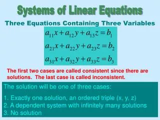
Problem Definition • We want to solve the problemwhere x is the vector of unknowns, while A and b are given • Assumptions • The number of equations is equal to the number of unknowns, therefore A is a square matrix • All components of A, b and x are real • A solution exists and it is unique • A-1 exists • A is not singular • A’s columns are linearly independent • A’s rows are linearly independent • det(A) is non-zero • rank(A) is equal to n • Ax = 0 only if x is a null vector Daniel Baur / Numerical Methods for Chemical Engineers / Linear Equation Systems
Analytical Approach • Cramer’s rule (1750):The solution is given bywhere Ai is defined as follows b replaces the ith column Daniel Baur / Numerical Methods for Chemical Engineers / Linear Equation Systems
Calculation of the Determinant • The Laplace formula (1772) allows the computation of the determinant of a square matrix: • where Ci,jis the determinant of the sub-matrix obtained by removing the ith row and the jth column of the matrix, multiplied by (-1)i+j: no jth column no ith row Daniel Baur / Numerical Methods for Chemical Engineers / Linear Equation Systems
A First Numerical Approach: Gauss Elimination Method • The following operations do not change the result: • Multiply a line by a constant • Substitute a line with a linear combination of multiple lines • Permute the order of lines • This can be used to produce a triangular matrix, which allows the solution to be found easily by substitution • Example system Daniel Baur / Numerical Methods for Chemical Engineers / Linear Equation Systems
Multiply by -3 • Sum it to 1st line • Multiply by -3 • Sum it to 1st line • Multiply by -4 • Sum it to 2nd line Triangular System Gauss Elimination Example Daniel Baur / Numerical Methods for Chemical Engineers / Linear Equation Systems
Generalization of the Gauss Elimination Method • We want to find a general procedure to replace one entry in the matrix with a zero; for this we define a multiplier l21 • Note that Daniel Baur / Numerical Methods for Chemical Engineers / Linear Equation Systems
The Gauss Elimination in Matrix Notation • If we put all multipliers for one column in one matrix, we getwhere • This way, a triangular matrix is easily obtained Daniel Baur / Numerical Methods for Chemical Engineers / Linear Equation Systems
Example: Gauss Elimination in Matrix Notation Total number of operations required (n-1)(n-2) operations (flops) n(n-1) operations (flops) Daniel Baur / Numerical Methods for Chemical Engineers / Linear Equation Systems
Gauss Elimination / Transformation Method • The Gauss elimination method is relatively easy to implement (even by hand), but has some distinct disadvantages; namely it • Changes the matrix A • Requires and changes the coefficient vector b • Must be rerun if the vector b changes • If we consider the Gauss method in matrix form on the other hand, we can see that we can useto transform A and b; M is therefore called the Gauss transformation matrix Daniel Baur / Numerical Methods for Chemical Engineers / Linear Equation Systems
The Gauss Transformation Method • We have so far • The final matrix A, which is an right triangular matrix • The matrix M, which is a left triangular matrix • The inverse of M is also a left triangular matrix Daniel Baur / Numerical Methods for Chemical Engineers / Linear Equation Systems
LR (LU) Factorization • We define our (right triangular) solution matrix as follows • If we multiply with L = M-1 from the left on both sides Daniel Baur / Numerical Methods for Chemical Engineers / Linear Equation Systems
LR Factorization (Continued) • The starting matrix A is transformed (factorized) as • If we apply this to a linear equation system, we get • This approach rids us of the disadvantages discussed earlier, because • For every vector b, two simple triangular systems must be solved without factorizing again • The matrices L and R can be stored using the elements of A • If A is modified, it is often possible to modify L and R accordingly without re-factorizing • Note that Gauss elimination is still needed once to compute L and R Daniel Baur / Numerical Methods for Chemical Engineers / Linear Equation Systems
Pivoting • It is easy to see from the definition of the multiplication factors, that the diagonal elements at each step (the pivot values) cannot be equal to zero • This is circumvented by reordering the rows of the matrix A by multiplication with a permutation matrix P • This approach is referred to as LRP-factorization(or LR-factorization with partial pivoting) • Example:a11 = 0 switch the lines x1 = x2 = 1 Daniel Baur / Numerical Methods for Chemical Engineers / Linear Equation Systems
Pivoting (Continued) • Pivoting must also take into account scaling problems;Let us consider a similar example • Pivot elements should have large absolute values Daniel Baur / Numerical Methods for Chemical Engineers / Linear Equation Systems
How does Matlab do it? • When using left divide \, Matlab chooses a procedure depending on the properties of the problem, i.e. if A is • Diagonal, x is computed directly by division • Sparse, square and banded, then banded solvers are used; Either Gauss elimination without pivoting or LR factorization • Left or right triangular, then backsubstitution is used • A permutation of a triangular matrix, it is permuted and 3. applies • Symmetric or Hermitian, then a Cholesky factorization is attempted (A = RR*, where R* is the conjugate transpose of R); If it fails, another indefinite symmetric factorization is attempted • Square but 1 through 5 do not apply, then LR factorization with partial pivoting is applied • Not square, then Householder reflections are used to compute a factorization which leads to a least-squares solution, i.e. a vector x which minimizes the length of Ax – b Daniel Baur / Numerical Methods for Chemical Engineers / Linear Equation Systems
Assignment 1 • Find online the template for an LR-factorization of a matrix with partial pivoting. Make the function operational by adding the lines that calculate the M matrix of the current step and the new A matrix. • Why does the transformation matrix T appear in the formula for M? Explain by comparing to the definition of M in the non-pivoting case. • Use the function to factorize the following matrix • Test if the factorization worked, i.e. if LR = A. • Is L in the form you would expect it to be? What implications does this have for its application in solving a linear system (see slide 13) and how could you correct for it? Daniel Baur / Numerical Methods for Chemical Engineers / Linear Equation Systems
Hints Daniel Baur / Numerical Methods for Chemical Engineers / Linear Equation Systems
Assignment 2 • Create a random matrix A with dimensions 4x4 and a random column vector b with size 4x1. Solve the system Ax = b. • Create a function that computes the determinant of square matrices using the Laplace formula. Use a recursive approach (see hints). • Use this function to compute the solution of the linear system above using Cramer’s rule. • Do the same for linear equation systems with sizes ranging from 5 to 9. • Read out the CPU time required to solve all these systems with both methods (Cramer’s method and A\b) and compare them. Daniel Baur / Numerical Methods for Chemical Engineers / Linear Equation Systems
Hints • If you remember the Laplace formula as a sumyou can see that the calculation of the determinant requires the calculation of a determinant. You could let the function call itself to do that (recursive function). Remember that the determinant of a 1x1 matrix is equal to its only element. • There are several Matlab commands to read out timings, however the most reliable one is • t_start = tic;statements;t_elapsed = toc(t_start); • Where the time elapsed (in second) is stored in t_elapsed Daniel Baur / Numerical Methods for Chemical Engineers / Linear Equation Systems