Unit 6: Comparing Two Populations or Groups
170 likes | 325 Views
Unit 6: Comparing Two Populations or Groups. Section 11.2 Comparing Two Means. Unit 6 Comparing Two Populations or Groups. 12.2 Comparing Two Proportions 11.2 Comparing Two Means. Section 11.2 Comparing Two Means. Learning Objectives. After this section, you should be able to…

Unit 6: Comparing Two Populations or Groups
E N D
Presentation Transcript
Unit 6: Comparing Two Populations or Groups Section 11.2 Comparing Two Means
Unit 6Comparing Two Populations or Groups • 12.2 Comparing Two Proportions • 11.2 Comparing Two Means
Section 11.2Comparing Two Means Learning Objectives After this section, you should be able to… • PERFORM a significance test to compare two means • INTERPRET the results of inference procedures
An observed difference between two sample means can reflect an actual difference in the parameters, or it may just be due to chance variation in random sampling or random assignment. Significance tests help us decide which explanation makes more sense. The null hypothesis has the general form H0: µ1 - µ2= hypothesized value We’re often interested in situations in which the hypothesized difference is 0. Then the null hypothesis says that there is no difference between the two parameters: H0: µ1 - µ2 = 0 or, alternatively, H0: µ1 = µ2 The alternative hypothesis says what kind of difference we expect. Ha: µ1 - µ2 > 0, Ha: µ1 - µ2 < 0, or Ha: µ1 - µ2 ≠ 0 Comparing Two Means • Significance Tests for µ1 – µ2 If the Random, Normal, and Independent conditions are met, we can proceed with calculations.
Comparing Two Means • Significance Tests for µ1 – µ2 To find the P-value, use the t distribution with degrees of freedom given by technology or by the conservative approach (df = smaller of n1- 1 and n2- 1).
Comparing Two Means • Two-Sample t Test for The Difference Between Two Means • If the following conditions are met, we can proceed with a two-sample t test for the difference between two means: Two-Sample tTest for the Difference Between Two Means
Comparing Two Means • Example: Calcium and Blood Pressure Does increasing the amount of calcium in our diet reduce blood pressure? Examination of a large sample of people revealed a relationship between calcium intake and blood pressure. The relationship was strongest for black men. Such observational studies do not establish causation. Researchers therefore designed a randomized comparative experiment. The subjects were 21 healthy black men who volunteered to take part in the experiment. They were randomly assigned to two groups: 10 of the men received a calcium supplement for 12 weeks, while the control group of 11 men received a placebo pill that looked identical. The experiment was double-blind. The response variable is the decrease in systolic (top number) blood pressure for a subject after 12 weeks, in millimeters of mercury. An increase appears as a negative response Here are the data: State: We want to perform a test of H0: µ1 - µ2 = 0 Ha: µ1 - µ2 > 0 where µ1= the true mean decrease in systolic blood pressure for healthy black men like the ones in this study who take a calcium supplement, and µ2= the true mean decrease in systolic blood pressure for healthy black men like the ones in this study who take a placebo. We will use α = 0.05.
Plan: If conditions are met, we will carry out a two-sample t test for µ1- µ2. • Random The 21 subjects were randomly assigned to the two treatments. • Normal With such small sample sizes, we need to examine the data to see if it’s reasonable to believe that the actual distributions of differences in blood pressure when taking calcium or placebo are Normal. Hand sketches of calculator boxplots and Normal probability plots for these data are below: The boxplots show no clear evidence of skewness and no outliers. The Normal probability plot of the placebo group’s responses looks very linear, while the Normal probability plot of the calcium group’s responses shows some slight curvature. With no outliers or clear skewness, the t procedures should be pretty accurate. • Independent Due to the random assignment, these two groups of men can be viewed as independent. Individual observations in each group should also be independent: knowing one subject’s change in blood pressure gives no information about another subject’s response. Comparing Two Means • Example: Calcium and Blood Pressure
Comparing Two Means • Example: Calcium and Blood Pressure Do: Since the conditions are satisfied, we can perform a two-sample t test for the difference µ1 – µ2. P-value Using the conservative df = 10 – 1 = 9, we can use Table B to show that the P-value is between 0.05 and 0.10. Conclude: Because the P-value is greater than α = 0.05, we fail to reject H0. The experiment provides some evidence that calcium reduces blood pressure, but the evidence is not convincing enough to conclude that calcium reduces blood pressure more than a placebo.
We can estimate the difference in the true mean decrease in blood pressure for the calcium and placebo treatments using a two-sample t interval for µ1 - µ2. To get results that are consistent with the one-tailed test at α = 0.05from the example, we’ll use a 90% confidence level. The conditions for constructing a confidence interval are the same as the ones that we checked in the example before performing the two-sample t test. With df = 9, the critical value for a 90% confidence interval is t* = 1.833. The interval is: Comparing Two Means • Example: Calcium and Blood Pressure We are 90% confident that the interval from -0.754 to 11.300 captures the difference in true mean blood pressure reduction on calcium over a placebo. Because the 90% confidence interval includes 0 as a plausible value for the difference, we cannot reject H0: µ1 - µ2 = 0 against the two-sided alternative at the α = 0.10 significance level or against the one-sided alternative at the α = 0.05 significance level.
The two-sample t procedures are more robust against non-Normality than the one-sample t methods. When the sizes of the two samples are equal and the two populations being compared have distributions with similar shapes, probability values from the t table are quite accurate for a broad range of distributions when the sample sizes are as small as n1= n2= 5. Comparing Two Means • Using Two-Sample t Procedures Wisely Using the Two-Sample tProcedures: The Normal Condition • Sample size less than 15: Use two-sample t procedures if the data in both samples/groups appear close to Normal (roughly symmetric, single peak, no outliers). If the data are clearly skewed or if outliers are present, do not use t. • Sample size at least 15: Two-sample t procedures can be used except in the presence of outliers or strong skewness. • Large samples: The two-sample t procedures can be used even for clearly skewed distributions when both samples/groups are large, roughly n ≥ 30.
Here are several cautions and considerations to make when using two-sample t procedures. Comparing Two Means • Using Two-Sample t Procedures Wisely • In planning a two-sample study, choose equal sample sizes if you can. • Do not use “pooled” two-sample t procedures! • We are safe using two-sample t procedures for comparing two means in a randomized experiment. • Do not use two-sample t procedures on paired data! • Beware of making inferences in the absence of randomization. The results may not be generalized to the larger population of interest.
Section 11.2Comparing Two Means Summary • Since we almost never know the population standard deviations in practice, we use the two-samplet statistic • where t has approximately a t distribution with degrees of freedom found by technology or by the conservative approach of using the smaller of n1 – 1 and n2 – 1 . • The conditions for two-sample t procedures are:
Section 11.2Comparing Two Means Summary • To test H0: µ1 - µ2= hypothesized value, use a two-sample t test for µ1 - µ2. The test statistic is P-values are calculated using the t distribution with degrees of freedom from either technology or the conservative approach.
Section 11.2Comparing Two Means Summary • The two-sample t procedures are quite robust against departures from Normality, especially when both sample/group sizes are large. • Inference about the difference µ1 - µ2in the effectiveness of two treatments in a completely randomized experiment is based on the randomization distribution of the difference between sample means. When the Random, Normal, and Independent conditions are met, our usual inference procedures based on the sampling distribution of the difference between sample means will be approximately correct. • Don’t use two-sample t procedures to compare means for paired data.
Homework: Chapter 11, #’s 40b, 41a, 42a, 43, 47a&b