Download
1 / 56
560 likes | 732 Views
KVANLI PAVUR KEELING. Concise Managerial Statistics. Chapter 11 – Comparing Two or More Populations. Slides prepared by Jeff Heyl Lincoln University. ©2006 Thomson/South-Western. Independent Versus Dependent Samples.

E N D
KVANLI PAVUR KEELING Concise Managerial Statistics Chapter 11 –Comparing Two or More Populations Slides prepared by Jeff Heyl Lincoln University ©2006 Thomson/South-Western
Independent VersusDependent Samples • Independent SamplesThe occurrence of an observation in the first sample has no effect on the value(s) in the other sample • Dependent Samples or paired samplesThe occurrence of an observation in the first sample has an impact on the corresponding value in the second sample
Dependent Samples • Comparisons of before versus after • Comparisons of people with matching characteristics • Comparisons of observations matched by location • Comparison of observations matched by time
2 1 Population 1 Population 2 µ2 µ1 Example of Two Populations Figure 11.1
For large samples where ’s are known (X1 - X2) - (µ1 - µ2) 2 2 n1n2 Z = 1 2 + The (1 - ) • 100 confidence interval 2 2 n1n2 2 2 n1n2 1 2 1 2 + + (X1 - X2) - Z/2 to (X1 - X2) + Z/2 Constructing a Confidence Interval for µ1 - µ2
Area = .90 Area = .45 Area = .45 Area = . 5 - .45 = .05 Area = . 5 - .45 = .05 Z -1.645 Z.05 = 1.645 Finding the Pair of Z Values Figure 11.2
Female heights (population 1) Male height (population 2) µ2 µ1 Example of Two Populations Figure 11.3
Approximate the standard normal random variable: (X1 - X2) 2 2 n1n2 Z = 1 2 + Hypothesis Testing for µ1 and µ2 (Large Samples)
2. Define the test statistic (X1 - X2) 2 2 n1n2 Z = 1 2 + Ace Delivery Example 1. Define the hypothesis Ho: µ1 ≤ µ2 (Texgas is less expensive) Ha: µ1 > µ2 (Quik-Chek is less expensive) Example 11.2
4. Evaluate the test statistic and carry out the tests (X1 - X2) 2 2 n1n2 (1.48 - 1.39) (.12)2 (.10)2 35 40 1 2 Z* = = = 3.50 + + Ace Delivery Example 3. Define the rejection region reject Ho if Z > 1.645 Example 11.2
Ace Delivery Example 5. State the conclusion Quik-Chek stores do charge less for gasoline (on the average) than do the Texgas stations Example 11.2
Area = . 5 - .05 = .45 Area = .05 Z k= 1.645 Z Curve of Rejection Region Figure 11.4
From Table A.4, area = .4998 Area = p = .5 - .4998 = .0002 Z Z*= 3.50 Z Curve with p-Value Figure 11.5
Two-Tailed Test Ho: µ1 = µ2 Ha: µ1 ≠ µ2 RejectHO if |Z| > Z/2 where (X1 - X2) 2 2 n1n2 Z = 1 2 + Independent Sample Tests for µ1 and µ2
One-Tailed Test Ho: µ1 ≤ µ2 Ha: µ1 > µ2 RejectHo if Z > Z Ho: µ1 ≥ µ2 Ha: µ1 < µ2 RejectHo if Z < - Z Independent Sample Tests for µ1 and µ2
Two-tailed hypotheses for independent sample tests Ho: µ1 - µ2 = D0 Ha: µ1 - µ2 ≠ D0 Right-sided one-tailed hypotheses Ho: µ1 - µ2 ≤ D0 Ha: µ1 - µ2 > D0 Two-Sample Procedure for Any Specified Value of µ1 - µ2
Test statistic is (X1 - X2) - Do 2 2 n1n2 Z = 1 2 + Two-Sample Procedure for Any Specified Value of µ1 - µ2
Two-Sample Z Test Figure 11.6
The df are given by df for t′= 2 s2s2 n1n2 1 2 2 2 s2 n2 s2 n1 + 1 2 + n1 - 1 n2 - 1 Test Statistic for µ1 - µ2 (Independent Samples)not assuming equal sigmas Approximately a t distribution defined as X1 - X2 - (µ1 - µ2) s2s2 n1n2 t′ = 2 1 +
A (1 - ) • 100% confidence interval is s2s2 n1n2 s2s2 n1n2 2 2 1 1 (X1 - X2) - t/2,df to (X1 - X2) + t/2,df + + Confidence Interval for µ1 - µ2 (Independent Samples)
1. The hypotheses are Ho: µ1 = µ2 Ha: µ1 ≠ µ2 X1 - X2 s2s2 n1n2 t´ = 2 1 + 2. The test statistic is Hypothesis Testing for µ1 - µ2 (Independent Samples) Example 11.5
3. The rejection region will be reject Ho if |t´| > t/2,df = t.05,22 = 1.717 4. The value of the test statistic is 3.33 - 3.98 (.68)2 (.38)2 15 15 -.65 .20 t´* = = = -3.25 + Hypothesis Testing for µ1 - µ2 (Independent Samples) Example 11.5
Hypothesis Testing for µ1 - µ2 (Independent Samples) 5. There is a significant difference in the average blowout times for the two brands Example 11.5
Two-Sample t Test Figure 11.7
Two-Sample t Test Figure 11.8
Two-Sample t Test Figure 11.9
(n1 - 1)s1 + (n2 - 1)s2 n1 + n2 - 2 2 2 sp = 2 Equal Variances If we believe variances to be equal, we can combine the estimates from each sample into a pooled sample variance, more powerful test
X1 - X2 1 1 n1n2 X1 - X2 s2 s2 n1 n2 t = = p p sp + + Equal Variances Confidence intervals are easier to compute since the distribution exactly follows a t distribution The degrees of freedom are df = n1+n2-2
Two-Tailed t Test Figure 11.10
35 – 30 – 25 – 20 – 15 – 10 – 5 – 0 – Before After Frequency | 10.11 | 10.13 | 10.15 | 10.17 | 10.19 | 10.21 | 10.23 | 10.25 | 10.27 | 10.29 | 10.31 | 10.33 | 10.35 Diameter Two-Tailed t Test Figure 11.11
Two-Tailed t Test Figure 11.12
Two-Tailed t Test Figure 11.13
Two-Tailed t Test Figure 11.14
Look at the ratio of sample variances s1 s2 2 F = 2 Comparing VariancesAssumptions • Both populations are normal • The samples are independent
Population 1 Population 2 1 2 µ2 µ1 Comparing Variances Figure 11.15
s1 s2 2 F = 2 Comparing Variances Figure 11.16
Population 2 Population 1 Population 1 Population 2 1 > 2 1 < 2 Comparing Variances Figure 11.17
V1 V2 1 2 6 7 8 9 1 39.86 49.50 58.20 58.91 59.44 59.86 2 8.53 9.00 9.33 9.35 9.37 9.38 6 3.78 3.46 3.05 3.01 2.98 2.96 7 3.59 3.26 2.83 2.78 2.75 2.72 8 3.46 3.11 2.67 2.62 2.59 2.56 9 3.29 3.01 2.55 2.51 2.47 2.44 Using The F-Statistic Table Table 11.1
Area = .10 F 2.67 Comparing Variances Figure 11.18
Area = .10 F .336 Comparing Variances Figure 11.19
Two-Tail Test Ho: 1 = 2 Ha: 1 ≠ 2 s1 s2 2 F = 2 RejectHo if F > F/2,v ,v(right tail) or if F < F1- /2,v ,v(left tail) 1 2 1 2 wherev1 = n1− 1 and v2 = n2− 1 Hypothesis Test for 1 and 2
One-Tail Test Ho: 1 ≤ 2 Ha: 1 > 2 Ho: 1 ≥ 2 Ha: 1 < 2 s1 s2 s1 s2 2 2 F = F = 2 2 RejectHo if F > F,v ,v wherev1 = n1− 1 andv2 = n2− 1 RejectHo if F < F1- ,v ,v wherev1 = n1− 1 andv2 = n2− 1 1 2 1 2 Hypothesis Test for 1 and 2
Allied Manufacturing Example Figure 11.20
The F-values are 1 F.025,v ,v FR = F.025,v ,vandFL = 1 2 1 2 The confidence interval is s12/s22 FL s12/s22 FR to Confidence Interval for 12/22
Area = .025 Area = .025 F FL FR Comparing Variances Figure 11.21
Test statistic d sd / n X1 - X2 sd / n tD = = ∑d2 - (∑d)2/n n - 1 sd = Comparing Paired, Dependent Samples d = difference between paired samples µd = mean of the population differences
The (1 - ) • 100% confidence interval is d - t/2,n - 1 to d + t/2,n - 1 sd n sd n Confidence Interval
Comparing Means Figure 11.22
Comparing Means Figure 11.23
Comparing Means Figure 11.24