WEEK 11 Graphs III A Simple Maximum-Flow Algorithm
WEEK 11 Graphs III A Simple Maximum-Flow Algorithm. CE222 – Data Structures & Algorithms II Chapter 9.4 (based on the book by M. A. Weiss, Data Structures and Algorithm Analysis in C++, 3rd edition, 2006 ). Network Flow Problems.


WEEK 11 Graphs III A Simple Maximum-Flow Algorithm
E N D
Presentation Transcript
WEEK 11Graphs IIIA Simple Maximum-Flow Algorithm CE222 – Data Structures & Algorithms II Chapter 9.4 (based on the book by M. A. Weiss, Data Structures and Algorithm Analysis in C++, 3rd edition, 2006)
Network Flow Problems Given a directed graph G=(V, E) with edge capacities cvw for each edge (v, w) We have 2 special vertices: s, which we call the source t, which is the sink. cvw v w CE 222-Data Structures & Algorithms II, Izmir University of Economics
Network Flow Problems Through any edge (v, w), at most cvw units of flow may pass. At any vertex, v, that is not either s or t, the total flow coming in must equal the total flow going out. CE 222-Data Structures & Algorithms II, Izmir University of Economics
20 2 4 10 30 s t 15 40 1 6 35 20 25 3 5 35 Problem Definition Maximum Flow Problem: Given a directed network G with edge capacities given by cvw’s, determine the maximum amount of flow that can be sent from a source node s to a sink node t. CE 222-Data Structures & Algorithms II, Izmir University of Economics
A Simple Maximum-Flow Algorithm Initial Attempt FlowgraphGftellstheflowattained at anystage. Initiallyalledges in Gfhave no flow (costs=0). Residualgraph Gr tells, foreachedge, howmuchmoreflow can be added (capacity - currentflow). An edge in Gr is known as a residualedge. Gr = G-Gf G Gf Gr CE 222-Data Structures & Algorithms II, Izmir University of Economics
A Simple Maximum-Flow Algorithm Initial Attempt Find a path in Gr from s to t. This path is known as an augmenting path. The minimum cost edge on this path is the amount of flow that can be added to every edge on the corresponding path in Gf. (Do this by adjusting Gf and recomputing Gr) If there is no path from s to t in Gr, we terminate. CE 222-Data Structures & Algorithms II, Izmir University of Economics
A Simple Maximum-Flow Algorithm Example 1/2 Initial stages of the graph, flow graph and residual graph G, Gf, Gr after 2 units of flow added along s, b, d, t CE 222-Data Structures & Algorithms II, Izmir University of Economics
A Simple Maximum-Flow Algorithm – Example 2/2 G, Gf, Gr after 2 units of flow added along s, a, c, t Looks allright? G, Gf, Gr after 1 unit of flow added along s, a, d, t– algorithm terminates. CE 222-Data Structures & Algorithms II, Izmir University of Economics
A Simple Maximum-Flow Algorithm – Example G, Gf, Gr If initial action is to add 3 units of flow along s, a, d, t– algorithm terminates. !!!Not Deterministic If we were to choose s, a, d, t with 3 units of flow, algorithm would terminate right there. CE 222-Data Structures & Algorithms II, Izmir University of Economics
A simple Maximum-Flow Algorithm – Correct Version In order to make the algorithm work, we need to allow the algorithm to change its mind. To do this, for every edge (v, w) with flow fv,w in Gf, we will add an edge (w, v) in the residual graph Gr of capacity fv,w. In effect, we are allowing the algorithm to undo its decisions by sending flow back in the opposite direction. Surprisingly, it can be shown that if the edge capacities are rational numbers, this algorithm always terminates with a maximal flow. CE 222-Data Structures & Algorithms II, Izmir University of Economics
Maximum-Flow Algorithm, Correct Version (Ford-Fulkerson Algorithm), Example I CE 222-Data Structures & Algorithms II, Izmir University of Economics
A simple Maximum-Flow Algorithm Example II for Correct Version 1/2 G, Gf, Gr after 3 units of flow along s, a, d, t using correct algorithm. CE 222-Data Structures & Algorithms II, Izmir University of Economics
A simple Maximum-Flow Algorithm – Example II for Correct Version 2/2 G, Gf, Gr after 2 units of flow along s, b, d, a, c, t using correct algorithm. If the capacities are all integers and maximum flow is f, then, since each augmenting path increases the flow by at least 1, f stages suffice, and the total running time is O(f*|E|), since an augmenting path can be found in O(|V|+|E|) time by an unweighted shortest path algorithm. This is BAD!!! CE 222-Data Structures & Algorithms II, Izmir University of Economics
A simple Maximum-Flow Algorithm Time Complexity – 1/2 • The classic example of why this is bad. Max-flow is seen to be 2,000,000. Continually augmenting along a path that includes the edge connected by a and b were to occur repeatedly, 2,000,000 augmentations would be required, when we could get by with only 2. CE 222-Data Structures & Algorithms II, Izmir University of Economics
A simple Maximum-Flow Algorithm Time Complexity – 2/2 A simple method to get around this problem is to always choose the augmenting path that allows the largest increase in flow. If capmax is the maximum edge capacity, O(|E|*log (capmax)) augmentations will suffice. Since O(|E|*log|V|) time is used for finding augmenting paths(dijkstra) O(|E|2*log|V|*logcapmax) If capacities are small integers, this reduces to O(|E|2*log|V|). CE 222-Data Structures & Algorithms II, Izmir University of Economics
A simple Maximum-Flow Algorithm – Time Complexity – III (Extra Slide) • (by Edmonds-Karp #1)Idea: don't just choose an arbitrary path. Instead, pick a path you can push a lot of flow along. Two versions: (1.1) use maximum bottleneck path (path with largest residual capacity). (1.2) Define a "capacity threshold" c and then just try to find an s-t path of residual capacity >= c. Advantage of this: it takes linear time. Just do a DFS over edges of residual capacity >= c . How to set c? Set initial value by trying 1,2,4,8,... until we can no longer find such a path. So, c is guaranteed to be within a factor 2 of max bottleneck F. Then, as we run the algorithm (finding paths and pushing flow along them), once there is no longer a path in which all edges have residual capacity >= c, we just let c = c/2. This ensures that c is within a factor 2 of F . • Claim: Either way, this causes algorithm to make at most O(|E|*log F) iterations. So, the total time using version 1.2 is O(|E|2 log F). • Proof of Claim: First, if the current residual graph has max flow f, then if we drop all edges of residual capacity < f/|E|, there must still exist a path from s to t (why? because let A be the component containing s. If A doesn't have t, then since there at most |E| edges out of A, this would be a cut with size < f. Contradiction). So, max bottleneck path has capacity at least f/|E|, and (if using version 1.2) this means c is at least f/(2|E|). CE 222-Data Structures & Algorithms II, Izmir University of Economics
A simple Maximum-Flow Algorithm – Time Complexity – IV (Extra Slide) • Let's just focus on version 1.2 (since then 1.1 follows directly). We have c is at least f/(2|E|). So can have at most 2*|E| iterations before c gets cut down by a factor of 2. Since c <= F at the start, we can cut down c at most log(F) times, so total number of iterations is at most 2|E|*log(F). Can we remove dependence on F completely? • (by Edmonds-Karp #2) Idea: always pick the shortest path (rather than the max-capacity path) Claim: this makes at most O(|E|*|V|) iterations. So, run time is O(E|2*|V|) since we use BFS in each iteration. Proof is pretty neat. Proof of Claim: Let d(t) be the distance from s to t in the current residual graph. We'll prove the theorem by showing that every |E| iterations, d(t) has to go up by at least 1. Let's lay out the graph in levels according to a BFS from s. Now, notice that so long as d(t) doesn't change, the paths found will only use forward edges. Each iteration saturates (and removes) at least 1 forward edge, and adds only backward edges (so no distance ever drops). This can happen at most |E|- d(t)+1 <= |E| times since after that many time, t would become disconnected from s. So, after |E| iterations, either t is disconnected (and d(t) = infinity) or else we must have used a non-forward edge, implying that d(t) has gone up by 1. Since d(t) can increase at most |V| times, there are at most O(|E|*|V|) iterations. CE 222-Data Structures & Algorithms II, Izmir University of Economics
Homework Assignments • 9.11, 9.12, 9.14, 9.41 • You are requested to study and solve the exercises. Note that these are for you to practice only. You are not to deliver the results to me. Izmir University of Economics