Maximum Flow
Maximum Flow. Maximum Flow Problem The Ford-Fulkerson method Maximum bipartite matching. material coursing through a system from a source to a sink. 12. 20. 16. s. t. 7. 9. 10. 4. 4. 13. 14. Flow networks:.

Maximum Flow
E N D
Presentation Transcript
Maximum Flow • Maximum Flow Problem • The Ford-Fulkerson method • Maximum bipartite matching
12 20 16 s t 7 9 10 4 4 13 14 Flow networks: • A flow network G=(V,E): a directed graph, where each edge (u,v)E has a nonnegative capacity c(u,v)>=0. • If (u,v)E, we assume that c(u,v)=0. • two distinct vertices :a source s and a sink t.
Flow: • G=(V,E): a flow network with capacity function c. • s-- the source and t-- the sink. • A flow in G: a real-valued function f:V*V R satisfying the following two properties: • Capacity constraint: For all u,v V, we require f(u,v) c( u,v). • Flow conservation: For all u V-{s,t}, we require
Net flow and value of a flow f: • The quantity f (u,v) is called the net flow from vertex u to vertex v. • The value of a flow is defined as • The total flow from source to any other vertices. • The same as the total flow from any vertices to the sink.
s t 12/12 15/20 11/16 10 1/4 4/9 7/7 8/13 4/4 11/14 A flow f in G with value .
Maximum-flow problem: • Given a flow network G with source s and sink t • Find a flow of maximum value from s to t. • How to solve it efficiently?
The Ford-Fulkerson method: • This section presents the Ford-Fulkerson method for solving the maximum-flow problem.We call it a “method” rather than an “algorithm” because it encompasses several implementations with different running times.The Ford-Fulkerson method depends on three important ideas that transcend the method and are relevant to many flow algorithms and problems: residual networks,augmenting paths,and cuts. These ideas are essential to the important max-flow min-cut theorem,which characterizes the value of maximum flow in terms of cuts of the flow network.
Continue: • FORD-FULKERSON-METHOD(G,s,t) • initialize flow f to 0 • while there exists an augmenting path p • doaugment flow f along p • return f
Residual networks: • Given a flow network and a flow, the residual network consists of edges that can admit more net flow. • G=(V,E) --a flow network with source s and sink t • f: a flow in G. • The amount of additional net flow from u to v before exceeding the capacity c(u,v) is the residual capacity of (u,v), given by: cf(u,v)=c(u,v)-f(u,v) in the other direction: cf(v, u)=c(v, u)+f(u, v).
12 4/12 v1 v3 v1 v3 16 4/16 20 s 10 t 4 7 10 t 4 9 4/9 13 4 13 4/4 v2 v4 v2 v4 14 4/14 Example of residual network 20 s 7 (a)
8 12 v1 v3 20 4 4 4 4 10 t 7 13 10 4 v2 v4 4 Example of Residual network (continued) s 5 (b)
Fact 1: • Let G=(V,E) be a flow network with source s and sink t, and let f be a flow in G. • Let Gf be the residual network of G induced by f,and let f’ be a flow in Gf.Then, the flow sum f+f’ is a flow in G with value . • f+f’: the flow in the same direction will be added. the flow in different directions will be cnacelled.
Augmenting paths: • Given a flow network G=(V,E) and a flow f, an augmenting path is a simple path from s to t in the residual network Gf. • Residual capacity of p : the maximum amount of net flow that we can ship along the edges of an augmenting path p, i.e., cf(p)=min{cf(u,v):(u,v) is on p}. 2 3 1 The residual capacity is 1.
8 12 v1 v3 20 4 4 4 4 10 t 7 13 10 4 v2 v4 4 Example of an augment path (bold edges) s 5 (b)
The basic Ford-Fulkerson algorithm: • FORD-FULKERSON(G,s,t) • for each edge (u,v) E[G] • do f[u,v] 0 • f[v,u] 0 • while there exists a path p from s to t in the residual network Gf • do cf(p) min{cf(u,v): (u,v) is in p} • for each edge (u,v) in p • do f[u,v] f[u,v]+cf(p)
Example: • The execution of the basic Ford-Fulkerson algorithm. • (a)-(d) Successive iterations of the while loop: The left side of each part shows the residual network Gf from line 4 with a shaded augmenting path p.The right side of each part shows the new flow f that results from adding fp to f.The residual network in (a) is the input network G.(e) The residual network at the last while loop test.It has no augmenting paths,and the flow f shown in (d) is therefore a maximum flow.
12 4/12 v1 v3 v1 v3 16 4/16 20 s 10 t 4 7 10 t 4 9 4/9 13 4 13 4/4 v2 v4 v2 v4 14 4/14 20 s 7 (a)
8 4/12 12 v1 v3 v1 v3 20 7/20 4 11/16 4 4 4 s 10 t 7/7 4 t 7 7/10 4/9 13 10 4 13 4/4 v2 v4 v2 v4 4 11/14 s 5 (b)
12/12 v1 v3 11/16 15/20 s 7/7 10 1/4 t 4/9 8 v1 v3 5 8/13 4/4 13 v2 v4 4 11 11/14 4 s 7 7 t 3 11 5 3 13 4 v2 v4 11 (c)
12 v1 v3 5 5 11 4 15 s 7 t 11 3 5 3 8 12/12 4 v2 v4 v1 v3 11 11/16 19/20 s 7/7 10 1/4 t 9 12/13 4/4 v2 v4 11/14 5 (d)
7 12 v1 v3 5 1 19 s 3 t 11 1 9 3 4 12 v2 v4 11 (e)
Time complexity: • If each c(e) is an integer, then time complexity is O(|E|f*), where f* is the maximum flow. • Reason: each time the flow is increased by at least one. • This might not be a polynomial time algorithm since f* can be represented by log (f*) bits. So, the input size might be log(f*).
The Edmonds-Karp algorithm • Find the augmenting path using breadth-first search. • Breadth-first search gives the shortest path for graphs (Assuming the length of each edge is 1.) • Time complexity of Edmonds-Karp algorithm is O(VE2). • The proof is very hard and is not required here.
Maximum bipartite matching: • Bipartite graph: a graph (V, E), where V=LR, L∩R=empty, and for every (u, v)E, u L and v R. • Given an undirected graph G=(V,E), a matching is a subset of edges ME such that for all vertices vV,at most one edge of M is incident on v.We say that a vertex v V is matched by matching M if some edge in M is incident on v;otherwise, v is unmatched. A maximum matching is a matching of maximum cardinality,that is, a matching M such that for any matching M’, we have .
L R (b) L R (a) A bipartite graph G=(V,E) with vertex partition V=LR.(a)A matching with cardinality 2.(b) A maximum matching with cardinality 3.
Finding a maximum bipartite matching: • We define the corresponding flow network G’=(V’,E’) for the bipartite graph G as follows. Let the source s and sink t be new vertices not in V, and let V’=V{s,t}.If the vertex partition of G is V=L R, the directed edges of G’ are given by E’={(s,u):uL} {(u,v):u L,v R,and (u,v) E} {(v,t):v R}.Finally, we assign unit capacity to each edge in E’. • We will show that a matching in G corresponds directly to a flow in G’s corresponding flow network G’. We say that a flow f on a flow network G=(V,E) is integer-valued if f(u,v) is an integer for all (u,v) V*V.
L R (a) s t L R (b) (a)The bipartite graph G=(V,E) with vertex partition V=LR. A maximum matching is shown by shaded edges.(b) The corresponding flow network.Each edge has unit capacity.Shaded edges have a flow of 1,and all other edges carry no flow.
Continue: • Lemma . • Let G=(V,E) be a bipartite graph with vertex partition V=LR,and let G’=(V’,E’) be its corresponding flow network.If M is a matching in G, then there is an integer-valued flow f in G’ with value .Conversely, if f is an integer-valued flow in G’,then there is a matching M in G with cardinality . • Reason: The edges incident to s and t ensures this. • Each node in the first column has in-degree 1 • Each node in the second column has out-degree 1. • So each node in the bipartite graph can be involved once in the flow.
1 1 1 1 1 1 1 Residual network. Red edges are new edges in the residual network. The new aug. path is bold. Green edges are old aug. path. old flow=1.