Innovative Protein Structure Alignment Using Predicted Local Structure Segments
This paper presents a novel approach to align homologous proteins utilizing Predicted Local Structure Segments (PLSSs). Traditional sequence alignment becomes challenging due to increasing evolutionary distances among proteins. We introduce an algorithm that leverages the Nearest-Neighbor Method to find optimal paths in a network of PLSSs, enabling significant improvements in structural comparison. Our dynamic programming technique calculates the maximum similarity score for protein segments, highlighting the utility of the HOMSTRAD database for effective homologous protein alignment.


Innovative Protein Structure Alignment Using Predicted Local Structure Segments
E N D
Presentation Transcript
Segment alignment SEA Segment Alignment to Compare Protein SEA B89902010鄭智懷 B89902037黃敬強 B89902117胡書瑜 B89010 鄭智懷 B89037 黃敬強 B89117 胡書瑜
Introduction • Outline of the paper • Increasing evolutionary distance causes homologous proteins to be hard to compare on a sequence level… • We focus on the folds of the protein, PLSSs, LSSs…etc. • A new look at the local structure prediction • Network matching problem
Introduction • PLSS( Predicted Local Structure Segment ) • LSS( Local Structure Segment ) maximal structural of units that are shared by proteins with different folds. • Predicted by the “Nearest-Neighbor Method” • PLSS the LSS use the previous method
The Basic Idea • Start with an arbitrarily chosen vertex and try to add edges vertex-by-vertex • Let x denote the latest vertex that was added to the path. Pick the one that is closest to x, and add to the path the edge connecting x and this vertex. Repeat until all vertices are included • Connect the starting vertex and the last
14 12 7 10 13 8 6 5 9
Introduction “Nearest-Neighbor Method”
d/d0 >= + 1/2 Denote Li as the i-th longest edge in D. • d0 >= 2L1 • d0 >= 2 1<=k<=[n/2] d0 >= 2
Algorithm Given two networks of PLSSs, find two optimal paths from the source to the sink in each of the networks, whose corresponding PLSSs are most similar to each other. It does not follow the typical position-by-position alignment mode
Algorithm possible PLSSs bit level sequence No overlapped PLSSs another presentation( by arrows ) 我們要表達的是一個sequence可以換成用PLSS來表示這一個蛋白質結構。
Algorithm Definition: 23 4 567 8 9… the position of the first vertex in this segment 就EEEEE來看 the position of the last vertex in this segment
Algorithm Definition: 23456789... A segment covers i, if 縮寫為 iα 就EEEEE來看 EEEEE covers 4,5,6,7,8
Algorithm Definition: 23456789... The set of PLSSs covering position i is denoted E(i). 就position=3來說 E(3) = {“EEE”,”HHHHHHHHHHH”}
Algorithm • The difference between original alignment and segment alignment • The same property between these two alignment ans: there are more than one possibility at position (i,j) . For any pair of positions, i and j, their covering segments are considered in a combinatorial way (total |E(i)|x|E(j)| combinations ). Here i and j are in the different sequence! ans: Using dynamic programming technique.
Algorithm • The idea: • Using dynamic programming concept 我們的目標是要找兩個PLSS sequence相似度最大(一個來自A;一個來自B),也就是把某一個PLSS sequence align到另一個PLSS sequence花最少的effort。在這樣的構想下我們便使用dynamic programming method to calculate the maximum score V(i,j). We define V(i,j ) as the maximum similarity score for transforming S1[1…i] to S2[1…j] calculated by
Algorithm • The NEW scoring scheme Δ( iα , jβ ) = WaΔ( Aai , Aaj )+ WsΔ( α , β) • Wa和Ws代表權重-> Wa + Ws = 1 • A是Blosum62 similarity matrix也就是一個scoring table 就如同上課所教的,給定兩個alphabets會return這兩個alphabet的分數。 這裡是給定sequence similarity defined by Blosum62 similarity matrix. • Δ( α , β)是另一個similarity matrix( scoring table ) from the HOMSTRAD database 這裡是給定兩個PLSS,return 這兩個PLSS的分數。 這裡是給定local structure similarity.
Algorithm • HOMSTRAD database (Homologous Structure Alignment Database) This database provides all known protein structure clustered into homologous families Using method: common ancestry
Algorithm • V(i,j) is the maximum similarity score for transforming S1[1,…,i] to S2[1,…,j] • V(iα,jβ) is the maximum similarity score for transforming S1[1,…,iα] to S2[1,…,jβ]
Algorithm The similarity score of aligned positions from (i-1, j-1) to (i, j) is ∆(iα,jβ) End with insertion 在這個位置已經存在deletion( insertion) gap再扣掉extension的分數 End with deletion 在這個位置的總分減掉開一個deletion gap的分數 看哪一個分數會比較高(在所有segment的可能下) g stands for the gap initiating penalty. h stands for the gap extension penalty.
Algorithm 代表前面一個位置一樣選α會有較高的分數(α之前出現過) 如果α第一次出現的位置是i則我們就要去考慮前面哪一個PLSS和α在一起的分數會最大 where 為什麼只須要考慮last(r) = i-1的呢?
Algorithm • 當r屬於E(i-1) & last(r) != i-1 代表這一個PLSS會cover到i,因為這一個PLSS cover i-1但是last(r) != i-1所以last(r) 會比 i-1 來的大,也就是說r會cover到i。這一種情形事實上已經被case 1所包括,因為case 1是對所有cover i 的PLSS,所以這個時候的 r 便是屬於case 1。
Complexity • 我們先假設dynamic programming每一個entry花的time complexity = O(1)。因為各做一次的substitution, insertion, deletion的時間複雜度是O(1)。 • 先假設的原因是有一些entry做的事不只是O(1),如果γ,δ是一個集合的話!
Complexity 我們先不失一般性的假設: In Sequence1 The first vertex 被a1個PLSS所cover (E(1)= a1) The second vertex 被a2個PLSS所cover (E(2)= a2) The third vertex 被a3個PLSS所cover (E(3)= a1) The m-1th vertex 被am-1個PLSS所cover (E(m-1)= am-1) The mth vertex 被am個PLSS所cover (E(m)= am) In Sequence2 The first vertex 被b1個PLSS所cover (E(1)=b1) The second vertex 被b2個PLSS所cover (E(2)=b2) The third vertex 被b3個PLSS所cover (E(3)=b3) The n-1th vertex 被bn-1個PLSS所cover (E(n-1)=bn-1) The nth vertex 被bn個PLSS所cover (E(n)= bn)
Complexity 在我們之前的假設下的time complexity In the i-row and j-column entity of the matrix do (ai)x (bj) operations So, the total operation in the matrix First row Second row Last row
Complexity • 先假設的原因是有一些entry做的事不只是O(1),如果γ,δ是一個集合的話! • 我們要證明γ,δ是一個集合時這種情形個數並不會太多。 • 當γ,δ是一個集合時,代表此PLSS是第一次出現在這一個位置,也就是說這種情形的個數=PLSS的個數。
Complexity 假設在sequence 1的PLSS個數是P1,在sequence 1的PLSS個數是P2。 則在做deletion時且γ是一個集合的總個數是NC1P1 同理 則在做insertion時且δ是一個集合的總個數是MC2P2 而substitution的總個數 = (#deletion) + (#insertion) 所以這一些的動作所須的time complexity = (#deletion) + (#insertion) NC1P1 +MC2P2 <= NC1M +MC2N <= MNC1C2 = O(MNC1C2)
Example: (1e68A,1nkl) <Residue-Number> specifies the number of a residue <Residue-Number>:<Residue-Number> selects all atoms that have residue numbers greater than or equal to the first residue number but less than or equal to the second residue number. 1e68A: Bacteriocin As-48 1nkl : Nk-lysin Residue Number
Example: (1e68A,1nkl) Each protein is represented as a collection of potentially overlapping and contradictory PLSSs (a network). SEA finds an optimal alignment between these two proteins Simultaneously, SEA identifies the optimal subset of PLSSs (a path in the network) describing each protein. 1e68A: Bacteriocin As-48 1nkl : Nk-lysin Residue Number
Several Variants of the SEA Algorithm • SEA_true: using segments derived from the actual 3D structure • SEA_cn: n is the maximum segment coverage(the numbers of segments that cover a position in each protein), ex: SEA_c30, SEA_c10, …etc. • SEA_1D: using 1D prediction (single predicted local structure)
General performance of SEA incorporating different local structure diversities CE(1998): Combinatorial Extension, combine a path defined by AFPs BLAST(1990), ALIGN(1988), FFAS(2000) are not computed from PLSS
General performance of SEA incorporating different local structure diversities Shift score: measure misalignment between a predicted alignment of two proteins and their reference alignment.
General performance of SEA incorporating different local structure diversities Shift Score gap Shift Score range from -0.2(epsilon) and 1.0 where e is a small number used as a parameter to the scoring algorithm
General performance of SEA incorporating different local structure diversities RMSD: root mean square deviation of C*alpha positions after optimal superposition (for structural similarity)
General performance of SEA incorporating different local structure diversities SEA_c30 and SEA_c10 produced most accurate alignments