Social Sub-groups

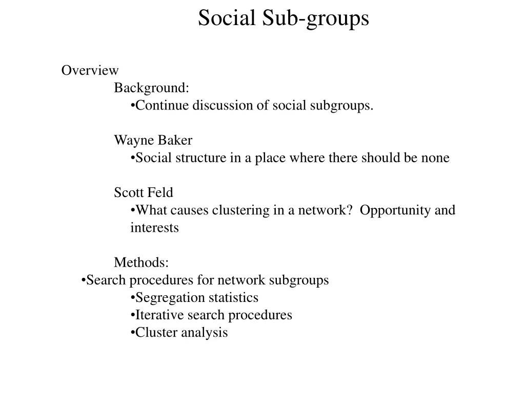
Social Sub-groups • Overview • Background: • Continue discussion of social subgroups. • Wayne Baker • Social structure in a place where there should be none • Scott Feld • What causes clustering in a network? Opportunity and interests • Methods: • Search procedures for network subgroups • Segregation statistics • Iterative search procedures • Cluster analysis

Social Sub-groups Wayne Baker: The Social Structure of a National Securities Market: 1) Behavioral assumptions of economic actors 2) Micro-structure of networks 3) Macro-structure of networks 4) Price Consequences Under standard economic assumptions, people should act rationally and act only on price. This would result in expansive and homogeneous (I.e. random) networks. It is, in fact, this structure that allows microeconomic theory to predict that prices will settle to an optimal equilibrium

Baker’s Model:

Baker’s Model: He makes two assumptions in contrast to standard economic assumptions: a) that people do not have access to perfect information and b) that some people act opportunistically He then shows how these assumptions change the underlying mechanisms in the market, focusing on price volatility as a marker for uncertainty. The key on the exchange floor is “market makers” people who will keep the process active, keep trading alive, and thus not ‘hoard’ (and lower profits system wide)

Baker’s Model: Micronetworks: Actors should trade extensively and widely. Why might they not? A) Physical factors (noise and distance) B) Avoid risk and build trust • Macro-Networks: Should be undifferentiated. Why not? • A) Large crowds should be more differentiated than small crowds. Why? • Price consequences: Markets should clear. They often don’t. Why? • Network differentiation reduces economic efficiency, leading to less information and more volatile prices

Baker: Use frequency of exchange to identify the network, resulting in: Baker finds that the structure of this network significantly (and differentially) affects the price volatility of the network

Baker: Because size is the primary determinant of clustering in this setting, he concludes that the standard economic assumption of large market = efficient is unwarranted.

Scott Feld: Focal Organization of Social Ties Feld wants to look at the effects of constraint & opportunity for mixing, to situate relational activity within a wider context. The contexts form “Foci”, “A social, psychological, legal or physical entity around which joint activities are organized” (p.1016) People with similar foci will be clustered together. He contrasts this with social balance theory. Claim: that much of the clustering attributed to interpersonal balance processes are really due to focal clustering. (note that this is not theoretically fair critique -- given that balance theory can easily accommodate non-personal balance factors (like smoking or group membership) but is a good empirical critique -- most researchers haven’t properly accounted for foci.)

Identifying Primary groups: 1) Measures of fit To identify a primary group, we need some measure of how clustered the network is. Usually, this is a function of the number of ties that fall within group to the number of ties that fall between group. 2) Algorithmic approaches to maximizing (1) Once we have such an index, we need a method for searching through the network to maximize the fit. We next go over various algorithms, that search different criteria for a fit. 3) Generalized cluster analysis In addition to maximizing a group function such as (1) we can use the relational distance directly, and look for clusters in the data. We next go over two different styles of cluster analysis

Measuring Cluster fit. • Many options. For a review, see: • Frank, K. A. 1995. "Identifying Cohesive Subgroups." Social Networks 1727-56. • Fershtman, M. 1997. "Cohesive Group Detection in a Social Network by the Segregation Matrix Index." Social Networks 19193-207 • Richards, William D. 1995. NEGOPY. Vers. 4.30. Brunaby, B.C. Canada Simon Fraser University.

Segregation Index (Freeman, L. C. 1972. "Segregation in Social Networks." Sociological Methods and Research 6411-30.) Freeman asked how we could identify segregation in a social network. Theoretically, he argues, if a given attribute (group label) does not matter for social relations, then relations should be distributed randomly with respect to the attribute. Thus, the difference between the number of cross-group ties expected by chance and the number observed measures segregation.

Segregation Index Consider the (hypothetical) network below. There are two attributes in this network: people with Blue eyes and Brown eyes and people who are square or not (they must be hip).

Blue Brown Blue 6 17 Brown 17 16 Hip Square Hip 20 3 Square 3 30 Segregation Index Mixing Matrix:

Segregation Index To calculate the number of expected, use the standard formula for a contingency table: Row marginal * column Marginal / Total observed Expected Blue Brown Blue 6 17 23 Brown 17 16 33 23 33 56 Blue Brown Blue 9.45 13.55 23 Brown 13.55 19.45 33 23 33 56 In matrix form: E(X) = R*C/T

Segregation Index observed Expected Blue Brown Blue 6 17 23 Brown 17 16 33 23 33 56 Blue Brown Blue 9.45 13.55 23 Brown 13.55 19.45 33 23 33 56 E(X) = (13.55+13.55) X = (17+17) Seg = 27.1 - 34 / 27.1 = -6.9 / 27.1 = -0.25

Segregation Index Observed Expected Hip Square Hip 20 3 23 Square 3 30 33 23 33 56 Blue Brown Blue 9.45 13.55 23 Brown 13.55 19.45 33 23 33 56 E(X) = (13.55+13.55) X = (3+3) Seg = 27.1 - 6 / 27.1 = 21.1 / 27.1 = 0.78

Segregation Index In SAS, you need to create a mixing matrix to calculate the segregation index. Mixmat.mod will do this. It does so using an indicator matrix. Blue 1 0 1 0 1 0 1 0 1 0 1 0 0 1 0 1 0 1 0 1 0 1 0 1 0 1 0 1 0 1 Square 0 1 0 1 0 1 1 0 1 0 1 0 1 0 1 0 1 0 0 1 0 1 0 1 0 1 0 1 0 1

Segregation Index You get the mixing matrix by pre multiplying the adjacency matrix by the transpose of the indicator matrix and post multiplying by the indicator matrix M = I`AI = I` A I M (k x k) (k x n)(n x n)(n x k)

Segregation Index In practice, how does the segregation index work? This is a plot of the extent of race segregation in a high school, by the racial heterogeneity of the high school

Segregation Index One problem with the segregation index is that it is not ‘margin free.’ That is, if you were to change the distribution of the category of interest (say race) by a constant but not the core association between race and friendship choice, you can get a different segregation level. One antidote to this problem is to use odds ratios. In this case, and odds ratio tells us the relative likelihood that two people in the same category will choose each other as friends.

Odds Ratios The odds ratio tells us how much more likely people in the same group are to nominate each other. You calculate the odds ratio based on the number of ties in a group and their relative size, based on the following table: Member of: Same Group Different Group Friends A B Not Friends C D OR = AD/ BC

Odds Ratios There are 6 hip people and 9 square people in this network. This implies that there are the following number of possible ties in the network: Observed Hip Square Hip 20 3 23 Square 3 30 33 23 33 56 Hip Square Hip 30 54 Square 54 72 Diagonal = ni(ni-1) off diagonal = ni2 Group Same Dif Yes 50 6 Friend No 52 102 OR = (50)102 / 52(6) = 16.35

Segregation index compared to the odds ratio: Friendship Segregation Index r=.95 Log(Same-Sex Odds Ratio)

Algorithms that maximize this type of fit (density / tie ratio based) • Factions in UCI-NET • Multiple options for the exact factor maximized. I recommend either the density or the correlation function, and I would calculate the distance in each case. • Frank’s KliqueFinder (the AJS paper we just read) • I have it, but I’ve yet to be able to get it to work. The folks at UCI-NET are planning on incorporating it into the next version. • Fershtman’s SMI • Never seen it programmed, though I use some of the ideas in the CROWDS algorithm discussed below

Factions Once you read your data into UCI-NET you can use factions, which in many ways is the easiest, though only if your networks are not too big.

Factions Input dataset: name of the network you want to cluster Fit criterion: Sum of the in-group ties Density of in-group ties Correlation of observed tie patterns to an ideal (block diagonal) “Other” - Steve Borgotti’s ‘special function’ - no idea what it means. Are diagonal’s valid? Depends on the data of interest Convert to geodesic: I recommend doing this if your network is fairly sparse Maximum # of iterations in a series: I usually go with the defaults. (Same with the next three options) Output: the name of the partition you want to save

Cluster analysis In addition to tools like FACTIONS, we can use the distance information contained in a network to cluster observations that are ‘close’ to each other. In general, cluster analysis is a set of techniques that allows you to identify collections of objects that are simmilar to each other in some degree. A very good reference is the SAS/STAT manual section called, “Introduction to clustering procedures.” (http://wks.uts.ohio-state.edu/sasdoc/8/sashtml/stat/chap8/index.htm) (See also Wasserman and Faust, though the coverage is spotty). We are going to start with the general problem of hierarchical clustering applied to any set of analytic objects based on similarity, and then transfer that to clustering nodes in a network.

Cluster analysis Imagine a set of objects (say people) arrayed in a two dimensional space. You want to identify groups of people based on their position in that space. How do you do it? How Smart you are How Cool you are

Cluster analysis Start by choosing a pair of people who are very close to each other (such as 15 & 16) and now treat that pair as one point, with a value equal to the mean position of the two nodes. x

Cluster analysis Now repeat that process for as long as possible.

Cluster analysis This process is captured in the cluster tree (called a dendrogram)

Cluster analysis • As with the network cluster algorithms, there are many options for clustering. The three that I use most are: • Ward’s Minimum Variance -- the one I use almost 95% of the time • Average Distance -- the one used in the example above • Median Distance -- very similar • Again, the SAS manual is the best single place I’ve found for information on each of these techniques. • Some things to keep in mind: • Units matter. The example above draws together pairs horizontally because the range there is smaller. Get around this by standardizing your data. • This is an inductive technique. You can find clusters in a purely random distribution of points. Consider the following example.

Cluster analysis The data in this scatter plot are produced using this code: data random; do i=1 to 20; x=rannor(0); y=rannor(0); output; end; run;

Cluster analysis Resulting dendrogram

Cluster analysis Resulting cluster solution

Cluster analysis Cluster analysis works by building a distance matrix between each pair of points. In the example above, it used the Euclidean distance which in two dimensions is simply the physical distance between the points in a plot. Can work on any number of dimensions. To use cluster analysis in a network, we base the distance on the path-distance between pairs of people in the network. Consider again the blue-eye hip example:

Cluster analysis Distance Matrix 0 1 3 2 3 3 4 3 3 2 3 2 2 1 1 1 0 2 2 2 3 3 3 2 1 2 2 1 2 1 3 2 0 3 2 4 3 3 2 1 1 1 2 2 3 2 2 3 0 1 1 2 1 1 2 3 3 3 2 1 3 2 2 1 0 2 1 1 1 1 2 2 3 3 2 3 3 4 1 2 0 1 1 2 3 4 4 4 3 2 4 3 3 2 1 1 0 2 2 2 3 3 4 4 3 3 3 3 1 1 1 2 0 1 2 3 3 4 3 2 3 2 2 1 1 2 2 1 0 1 2 2 3 3 2 2 1 1 2 1 3 2 2 1 0 1 1 2 2 2 3 2 1 3 2 4 3 3 2 1 0 1 2 2 3 2 2 1 3 2 4 3 3 2 1 1 0 1 1 2 2 1 2 3 3 4 4 4 3 2 2 1 0 2 2 1 2 2 2 3 3 4 3 3 2 2 1 2 0 1 1 1 3 1 2 2 3 2 2 2 3 2 2 1 0

Cluster analysis The distance matrix implies a space that nodes are embedded within. Using something like MDS, we can represent the space implied by the distance matrix in two dimensions. This is the image of the network you would get if you did that.

Cluster analysis When you use variables, the cluster analysis program generates a distance matrix. We can, instead use the network distance matrix directly. If we do that with this example network, we get the following:

Cluster analysis

Cluster analysis In SAS you use two commands to get a cluster analysis. The first does the hierarchical clustering. The second analyzes the cluster output to create the tree. Example 1. Using variables to define the space (like income and musical taste): procclusterdata=a method=ave out=clustd std; var x y; id node; run; proctreedata=clustd ncl=5out=cluvars; run;

Cluster analysis prociml; %include'c:\moody\sas\programs\modules\reach.mod'; /* blue eye example */ mat2=j(15,15,0); mat2[1,{21415}]=1; /* lines cut here */ mat2[15,{11424}]=1; dmat=reach(mat2); mattrib dmat format=1.0; print dmat; id=1:nrow(dmat); id=id`; ddat=id||dmat; create ddat from ddat; /* creates the dataset */ append from ddat; quit; data ddat (type=dist); /* tells SAS it is a distance */ set ddat; /*matrix*/ run; Example 2. Using a pre-defined distance matrix to define the space (as in a social network). You first create the distance matrix (in IML), then use it in the cluster program.

Cluster analysis Example 2. Using a pre-defined distance matrix to define the space (as in a social network). Once you have it, the cluster program is just the same. procclusterdata=ddat method=ward out=clustd; id col1; run; proctreedata=clustd ncl=3out=netclust; copy col1; run; procfreqdata=netclust; tables cluster; run; procprintdata=netclust; var col1 cluster; run;

The CROWDS algorithm combines the density approach above with an initial cluster analysis and a routine for determining how many clusters are in the network. It does so by using the Segregation index and all of the information from the cluster hierarchy, combining two groups only if it improves the segregation fit for both groups.

The one other program you should know about is NEGOPY. Negopy is a program that combines elements of the density based approach and the graph theoretic approach to find groups and positions. Like CROWDS, NEGOPY assigns people both to groups and to ‘outsider’ or ‘between’ group positions. It also tells you how many groups are in the network. It’s a DOS based program, and a little clunky to use, but NEGWRITE.MOD will translate your data into NEGOPY format if you want to use it. There are many other approaches. If you’re interested in some specifically designed for very large networks (10,000+ nodes), I’ve developed something I call Recursive Neighborhood Means that seems to work fairly well.

Social Sub-groups