Bivariate Data Prediction Techniques
Learn how to predict Y values using X values in bivariate data. Explore regression lines, slopes, intercepts, and error measurements.

Bivariate Data Prediction Techniques
E N D
Presentation Transcript
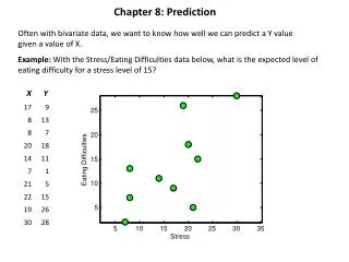
Chapter 8: Prediction Often with bivariate data, we want to know how well we can predict a Y value given a value of X. Example: With the Stress/Eating Difficulties data below, what is the expected level of eating difficulty for a stress level of 15? X Y 25 20 Eating Difficulties Eating Difficulties 15 10 5 5 10 15 20 25 30 35 Stress
Example: With the Stress/Eating Difficulties data below, what is the expected level of eating difficulty for a stress level of 15? The basic procedure is to draw the best-fitting line through the scatter plot, and find the value of Y corresponding to X=15. X Y 25 20 Y = ??? Eating Difficulties Eating Difficulties 15 10 X = 15 5 5 10 15 20 25 30 35 Stress What does it mean to be the ‘best-fitting line’?
A quick look back on the definitions of the mean and variance: It turns out that the mean is the value that minimizes the sums of squared deviations. This equation: is true for all values of a In other words, the mean is the ‘best-fitting’ value for the values of X in terms of the sums of squared deviations. Correspondingly, the best-fitting line is the line that minimizes the sums of squared differences between the line and each data point. This line is called the regression line.
Correspondingly, the best-fitting line is the line that minimizes the sums of squared differences between the line and each data point. This line is called the regression line. 25 20 Y = ??? Eating Difficulties Eating Difficulties 15 10 X = 15 5 5 10 15 20 25 30 35 Stress
Quick review on slopes and intercepts: The ‘point-slope’ formula for a line is: Y = m(X-x1)+y1 Where m is the slope, and (x1,y1) is a point on the line (x1,y1) m 1
The regression line passes through the means of X and Y : X Y 25 20 Y = ??? Eating Difficulties Eating Difficulties Eating Difficulties 15 10 X = 15 5 5 10 15 20 25 30 35 Stress
The slope of the regression line is: where r is the Pearson correlation SX and SY are the standard deviations of x and y Putting it together, the equation of the regression line is: Y-intercept slope
Calculating the regression line in our example Equation of regression line:
Original Example Question: What is the expected level of eating difficulty for a stress level of 15? Answer: Plug 15 in for X in the equation of the regression line: We expect an eating difficulty level of 12.02 for a stress level of 15 25 20 Y = 12.2 Eating Difficulties Eating Difficulties 15 10 X = 15 5 5 10 15 20 25 30 35 Stress
Another example: The ages of men and women in the US when they marry correlate with a value of r=0.85. Suppose that the average age at marriage for women is 25.1 years with a standard deviation of 5 years, and the average age at marriage for men is 26.8 years with a standard deviation of 6 years. What is the expected age of a groom for a 22 year old bride? (these numbers are made up) Answer: We need to calculate the regression line with X = women and Y = men, and evaluate it for X = 22. Plugging in 22 for X: The expected age of a groom for a 22 year old bride is 23.6 years.
50 40 30 20 10 0 10 20 30 40 50 r=0.85, Regression line: Y'=1.02X+1.20 Here’s what a typical sample of 200 couples would look like with r = 0.85 Age of Groom Y'=1.02X+1.20 Age of Bride
r=1.00, Regression line: Y'=1.20X-3.32 50 40 30 Age of Groom 20 10 r=0.00, Regression line: Y'=0.00X+26.8 0 0 20 40 40 Age of Bride 30 Age of Groom 20 10 20 30 40 Age of Bride Here are typical distributions for extreme values of r Correlation of r=1.0 Correlation of r=0.0 Look what happens to the regression line. When r=1, we can perfectly predict the groom’s age based entirely on the means and variances. When the correlation is zero, then we can’t say anything about the groom’s age based on the bride’s, so our best estimate is the mean age of the groom (26.8 years).
SYX: the standard error of the estimate The regression line is the ‘best-fitting’ line through a bivariate distribution in terms of minimizing the sums of squared deviations between the values of Y and the line. How can we measure how good this fit is? A natural measure is the standard error of the estimate: 25 (Y-Y’) 20 This is just like a standard deviation. It’s a measure of the average deviation between the line and the data. Eating Difficulties Eating Difficulties 15 10 X = 15 5 5 10 15 20 25 30 35 Stress
r=1 r=0 50 40 40 30 Age of Groom 30 Age of Groom 20 20 10 0 0 20 40 10 20 30 40 Age of Bride Age of Bride Another way of calculating SYXis: This makes intuitive sense. How well the data fits the line is a combination of the variability in Y (SY), and the correlation (r). If the correlation is perfect (r=1), then SYX = 0. If the correlation is zero, then SYX = SY. Notice that is SYXalways less than or equal to SY