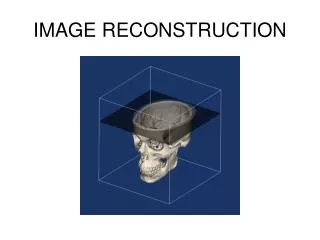
Image Reconstruction from Projections
Image Reconstruction from Projections. Antti Tuomas Jalava Jaime Garrido Ceca. Overview. Reconstruction methods Fourier slice theorem & Fourier method Backprojection Filtered backprojection Algebraic reconstruction Diffractive tomography Display of CT images


Image Reconstruction from Projections
E N D
Presentation Transcript
Image Reconstruction from Projections Antti Tuomas Jalava Jaime Garrido Ceca
Overview • Reconstruction methods • Fourier slice theorem & Fourier method • Backprojection • Filtered backprojection • Algebraic reconstruction • Diffractive tomography • Display of CT images • Tissue characterization with CT
Projection Geometry • Problem: Reconstructing 2D Image. • Given parallel-ray projections. • 1D projection (Radon transform). • Density distribution • Ray AB • Integral evaluated for different values of the ray offset t1. • 1D projection or Radon transform.
The Fourier Slice Theorem • 1D Fourier Transform of 1D projection of 2D image is equal to the radial section (slice or profile) of the2D Fourier Transform of the 2D image at the angle of the projection.
The Fourier Slice Theorem • How to obtain f(x,y) applying Fourier Slice Theorem: • Assumption: we have projections available at all angles from 0º to 180º. • From projections, we take their 1D Fourier transform. • Fill the 2D Fourier Space with the corresponding radial sections. • Take an inverse 2D Fourier transform to obtain • Problem: finite number of projections available • Solution: Interpolation is needed in 2D Fourier space.
Backprojection • Simplest reconstruction procedure • Assumptions: • Rays: Ideal straight lines. • Image: dimensionless points. • Procedure • Estimate of the density at a point by simply summing (integrating ) all the rays that pass through it at various angles. • Problem: • Finite number of rays per projection • Finite number of projections • Interpolation is required.
Backprojection • BP produces a spoke-line pattern blurring details. • Finite number of projections produces streaking artifacts. • Reconstructed image modeled by convolution between PSF (impulse response) and the original image. • Solution: • Applying deconvolution filters to the reconstructed image. • Filtered BP technique.
Filter is represented by this function: Ramp filter Filtered Backprojection • After some manipulations, we get: where • In practice, smoothing window should be applied to reduce the amplification of high-frequency noise.
Frequency axis discretized Finite number of samples Samples at the sampling rate 2W Discrete Filtered Backprojection • Projection in frequency domain is manipulated:
Problem: control noise enhancement • Solution we apply hamming window: Discrete Filtered Backprojection • The filtered projection may then be obtained as:
Discrete Filtered Backprojection • Finally, we get this expression : • Algorithmic: • Measure projection. • Compute filtered projection. • Backproject the filtered. • Repeat 1-3 all projection angles
Filtered back projection 10° Original Filtered back projection 1° Back projection 1°
Contribution factor of the nth image element to the mth ray sum. Algebraic Reconstruction Techniques • Projections seen as set of simultaneous equations. • Kaczmarz method • Iterative method. • Implemented easily. • Assumptions: • Discrete pixels. • Image density is constant within each cell. • Equations
Algebraic Reconstruction Techniques • Karzmarz method take the approach of successively and iteratively projecting an initial guess and its successors from one hyperplane to the next. • In general, the mth estimate is obtained from the (m-1)th estimate as: • Because the image is updated by altering the pixels along each individual ray sum, the index of the updated estimate or of the iteration is equal to the index of the latest ray sum used.
Algebraic Reconstruction Techniques • Characteristics worth: • ART proceed ray by ray and it is iterative • Small angles between hyperplanes • Large number or iterations • It should be reduced by using optimized ray-access schemes. • M>N noisy measurements oscillate in the neighborhood of the intersections of the hyperplanes. • M<N under-determined. • Any a priori information about image is easily introduced into the iterative procedure.
True ray sum Computed ray sum Number of pixels crossed by the mth ray. Approximations to the Kaczmarz method • We could rewrite reconstruction step at the nth pixel level as: • Corrections could also be multiplicative:
Approximations to the Kaczmarz method • Generic ART procedure: • Prepare an initial estimate • Compute ray sum • Obtain difference between true ray sum and the computed ray sum and apply the correction. • Perform Steps 2 and 3 for all rays available. • Repeat Steps 2-4 as many times as required.
Original 1. 178 angles dt = 1 voxel width 3. 2.
Original again 4. 5. 6.
Imaging with Diffraction Sources • Non ionizing radiation • Ultrasonic • Electromagnetic (optical or thermal) • Refraction and diffraction • Fourier diffraction theorem
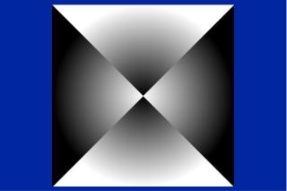
Imaging with Diffraction Sources When an object, f(x,y), is illuminated with a plane wave the Fourier transform of the forward scattered fields measured on line TT’ gives the values of the 2-D transform, F(w1,w2), of the object along a circular arc in the frequency domain, as shown in the right half of the figure.
Display of CT Images • = measured attenuation coefficient. • = attenuation coefficient of water • When K = 1000 units are called Hounsfield Units • Air: -1000 HU • Water: 0 HU • Bone 1000 HU • Study • 86 healthy infants aged 0-5 years • White matter: 15 HU to 22 HU • Gray matter: 23 HU to 30 HU • Difference between grey and white matter exactly 8 HU (In all measurements) • Boris P, Bundgaard F, Olsen A. Childs Nerv Syst. 1987;3(3):175-7
Microtomography • µ-scale CT • Volume: few • Nanotomography already introduced. • Biomedical use: • Both dead and alive (in-vivo) rat and mouse scanning. • Human skin samples, small tumors, mice bone for osteoporosis research.
Estimation of Tissue Components with CT • Manual segmentation of tumor by radiologist • Parametric model for the tissue composition • Gaussian mixture model • Method to estimate the parameters of the model • EM algorithm
Gaussian Mixture Model (i) • Fit M gaussian kernels to intensity histogram
Gaussian Mixture Model (ii) • Intensity value for voxel is a Gaussian random variable. • Parameters for ith tissue: • Probability that voxel belonging to that tissue gets value x • M number of different tissues in tumor • = the fraction of belonging to ith tissue (probability). • Tumor as whole: PDF is a mixture of M Gaussians
Gaussian Mixture Model (iii) • Tumor as whole: PDF is a mixture of M Gaussians • Probability of parameter set • If nothing is known about Find that maximizes likelihood
Gaussian Mixture Model (iv) • Probability that jth voxel with value belongs to the ith tissue type • EM algorithm (iterative, chapter 8) ->
Ending Remarks • Some image manipulation tasks can be performed in 1D in radon domain (edge detection etc.). • Reconstruction heavily dependent on reconstruction algorithm (method). • MRI images are usually reconstructed with Fourier method (according to book). • CT allows fast 3D imaging • So does MRI. MRI has better sensitivity especially with soft tissues.