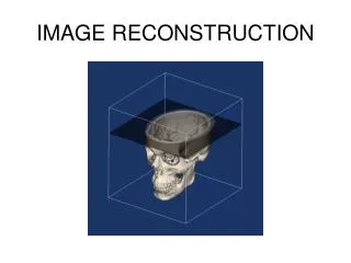
Image Reconstruction
Image Reconstruction. Image Reconstruction II. Generating an image from the acquired data involves determining the linear attenuation coefficients of the individual voxels. A mathematical algorithm takes the projection data and reconstructs the cross‑sectional CT image.
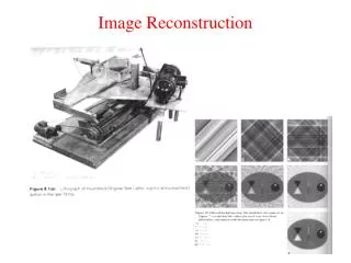

Image Reconstruction
E N D
Presentation Transcript
Image Reconstruction II Generating an image from the acquired data involves determining the linear attenuation coefficients of the individual voxels. A mathematical algorithm takes the projection data and reconstructs the cross‑sectional CT image. There are three common ways to carry this out: 1: Backprojection 2: Iterative 3: Fourier methods
Backprojection The field of view is simulated as a 2-D array within the computer. 512 x 512 The attenuation for each voxel of a scan is 1: projected back along the direction of the beam 2: the attenuation is added to the value in each array element the beam passes through. At the end of the procedure a rough image is held in the array elements.
Filtered Backprojection • No commercial CT scanners use simple back projection • The process produces artifacts where the attenuation changes rapidly. • Most modern scanners use filtered back projection algorithms • which have filter functions applied to reduce these effects. • Different filters may be used, offering tradeoffs • between spatial resolution and noise. • Some filters permit reconstruction of fine detail but with increased • noise in the image such as in bone algorithms. • Algorithms such as those for soft tissue provide some smoothing, • which decreases image noise but also decreases spatial resolution. • The choice of the best filter to use with the reconstruction algorithm • depends on the clinical task.
Image display Reconstructed images are viewed on CRT monitors or printed onto film using a laser printer. Each pixel is normally represented by 12 bits, or 4096 grey levels The normal grey levels available on a display are 256 Window width and window level are used to optimise the appearance of CT images by determining the contrast and brightness levels assigned to the CT image data . Window level, or centre, is the CT number or HU value to be displayed as the median intensity in the image. The window level is normally chosen close to the average HU value of the tissue of interest (e.g., 10 to 50 HU for soft tissue). Window width is the range of CT numbers displayed around the selected centre. and it determines the contrast. A narrow window width provides higher contrast than a wide window width.
Image Quality • Image quality may be characterised in terms of • contrast • noise • spatial resolution • Image quality involves tradeoffs between these three factors • and patient radiation dose. • Artifacts encountered during CT scanning can degrade image quality.
Contrast • The difference in the HU values between tissues. • Usually increases as kVp decreases • but is not affected by mA or scan times. • CT contrast may be artificially increased by adding a contrast medium • such as iodine. • Image noise may prevent detection of low‑contrast objects such • as tumours with a density close to the adjacent tissue. • The displayed image contrast is primarily determined by the CT • window width and window level settings.
Noise • CT noise is determined primarily by the number of photons • used to make an image (quantum mottle). • Quantum mottle decreases as the number of photons increases. • The typical noise with a modern CT system is approximately • 5 HU • CT noise is generally • reduced by increasing the • ·kVp, • ·mA • ·scan time • ·voxel size • (i.e., by decreasing matrix size, increasing FOV, • or increasing section thickness).
Resolution Typical resolution in CT scanning ranges from 0.7 to 1.5 lp/mm. If the CT Field Of View [FOV] is d and the matrix size is M, then the pixel size is d /M. For a typical head scan with an FOV of 25 cm A matrix of 512 pixels The pixel size is 0.5 mm. Factors that may also improve CT spatial resolution ·smaller focal spots ·smaller detectors · more projections. · smaller FOV · larger matrix size. Resolution perpendicular to the section is dependent on slice thickness
Radiation The dose profile in a CT scanner is not uniform along the patient axis and may vary within any irradiated section. Typical maximum doses for a single section are 40 mGy (4 rads) for a head scan 20 mGy (2 rads) for a body scan.
Radiation In head scans, the surface to centre ratio is approximately 1:1. In body scans, the surface to centre ratio is approximately 2:1.
Radiation Because of scattered x‑rays, the CT section dose profile is not perfectly square but has tails that extend beyond the section edges. Tissues beyond the section are thus exposed to radiation. When contiguous sections are scanned, the cumulative radiation dose in a section may be as high as twice the radiation dose associated with a single section.
Artifacts Partial volume artefact CT scanners may have artifacts in the reconstructed images. Partial volume artefact is the result of averaging the linear attenuation coefficient in a voxel that is not uniform in composition. Partial volume artefact increases with pixel size and section thickness.
Artifacts Streak Artifacts Random or unpredictable motion (e.g., if the patient sneezes) produces streak artifacts in the direction of motion. In high‑density structures, such as metal implants, the detector may record no transmission. The algorithm generates streaks adjacent to the high‑densities.
Artifacts Beam Hardening Artifacts Beam hardening artifacts or "cup" artifacts are caused by the polychromatic nature of the x‑ray beam (beam hardening). As the lower energy photons are preferentially absorbed, the beam becomes more penetrating and results in lower computed values of the attenuation coefficient (HU). Beam hardening artifacts are most marked at high‑contrast interfaces such as between dense bone in the skull and the brain
Artifacts Ring artifacts Ring artifacts may arise in third‑generation systems if a single detector is faulty or miscalibrated. Artifacts caused by equipment defects are rare on modern CT systems