Silicon Detector Readout
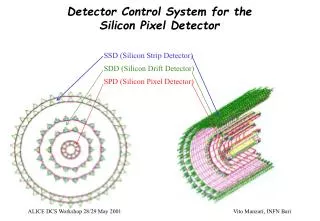
IPM-HEPHY Detector School. Silicon Detector Readout. 14 June 2012 Markus Friedl (HEPHY). Contents. Silicon Detector Front-End Amplifier Signal Transmission Back-End Signal Processing Summary. Example: CMS Experiment at CERN. Tracker (Silicon Strip & Pixel Detectors). CMS Tracker.

Silicon Detector Readout
E N D
Presentation Transcript
IPM-HEPHY Detector School Silicon DetectorReadout 14 June 2012 Markus Friedl (HEPHY)
Contents • Silicon Detector • Front-End Amplifier • Signal Transmission • Back-End Signal Processing • Summary M.Friedl: Silicon Detector Readout
Example: CMS Experiment at CERN Tracker(Silicon Strip & Pixel Detectors) M.Friedl: Silicon Detector Readout
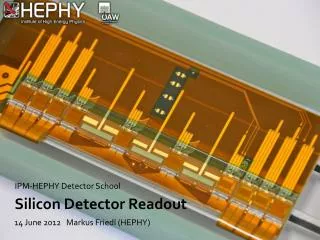
CMS Tracker Silicon Strip Sensor Front-End Electronics M.Friedl: Silicon Detector Readout
Silicon Detector • Front-End Amplifier • Signal Transmission • Back-End Signal Processing • Summary M.Friedl: Silicon Detector Readout
Various CMS Tracker Modules Electronics Sensors M.Friedl: Silicon Detector Readout
Silicon Strip Detectors Wire bond • Typically 300µm thick, strip pitch 50...200µm • Reverse bias voltage for full depletion 50...500V • Connection by wire bonds CMS Test Sensor with various geometries (1998) Belle Sensor with 45° strips (2004) M.Friedl: Silicon Detector Readout
Silicon Pixel Detectors • Pixels can be square (CMS) or oblong (ATLAS) • Structure size similar to strip detectors, but N2 channels • Connection by bump bonds CMS Pixel Readout Scheme CMS Pixel Sensor ATLAS Pixel Sensor M.Friedl: Silicon Detector Readout
Principle of Operation • p-n junction is operated at reverse bias to drain free carriers • Traversing charged particle creates electron-hole pairs • Carriers drift towards electrodes in the electric field • Moving carriers induce current in the circuit current source M.Friedl: Silicon Detector Readout
Equivalent Circuit of the Detector • Applies to many types of detectors, not only silicon • Example: wire chamber • Coaxial capacitor configuration • Moving charges induce current • Example: photomultiplier tube • Small plates • Charge (current) is amplified in each stage Current source with capacitor in parallel M.Friedl: Silicon Detector Readout
Comparison: Voltage vs. Current Source IDEAL REAL M.Friedl: Silicon Detector Readout
Moving Charges M.Friedl: Silicon Detector Readout
Ramo’s Theorem (1939) • Moving charges between inside electric field (e.g. parallel plates) induces current in electrodes i = E q v • Current is proportional to electric field E, (moving) charge q and velocity v of the charge • It doesn’t matter if the charges eventually reach the electrodes or not, only motion counts • Fully valid for parallel plate capacitor configuration (large area diode) • A bit more complicated for strip detectors more later M.Friedl: Silicon Detector Readout
A Bit of Theory • Space charge density is given by doping • Electric field is calculated by Poisson’s equation • Potential is found by integration of field • Shown here: full depletion = space charge just extends over full detector M.Friedl: Silicon Detector Readout
Bias Voltage and Depletion • In reality, the electric field is imposed by applied bias voltage • What happens if Vbias < Vdepl? • Electric field does not cover full bulk • Only part of detector contributes tocharge collection lower efficiency • Do not operate a detector like that • What happens if Vbias > Vdepl? • Linear offset is added to electric field • Field tends to become more flat • Faster charge collection (Ramo) • Limited by breakdown voltage M.Friedl: Silicon Detector Readout
Induced Currents (1) M.Friedl: Silicon Detector Readout
Induced Currents (2) • Typical silicon detector (D=300µm) • Very low (<1µA), very short (~20ns) • Different contributions from moving charges • Electrons have higher mobility, thus faster • Holes with lower mobility are slower • Exponential curves with (theoretically) infinite tail at V=Vdepl • Almost triangular shapes at V= 2 Vdepl due to flatter field M.Friedl: Silicon Detector Readout
Induced Currents (3) • Both electrons and holes contribute to overall current, but cannot be distinguished in reality • Integral over time (area under curve) is the collected charge • If all charges reach electrodes, this is identical to the number of created pairs • i dt ≈ 3.6 fC 22500 e for a 300µm thick detector • For comparison: ~1010 e every 20ns in a 25W bulb (230VAC) • In a simple parallel plate geometry, contributions of electrons and holes are equal • However, it’s not that simple in a strip detector… M.Friedl: Silicon Detector Readout
Induced Current Measurement • Quite difficult due to noise constraints • Every amplifier has a limited bandwidth and thus rise time • Nonetheless, exponential decay is clearly visible Single shot Averaged M.Friedl: Silicon Detector Readout
Strip Detector Case • Ramo theorem still holds, but with some modifications • Charge movement is determined by electric field (which is approximately the same as for the parallel plate case) • Induced currents are calculated by (virtual) weighting field • Why? • Now the moving charges influence a current onto several strips depending on the geometry and distance • How to calculate weighting field? • Electrode under consideration is held at unity potential, all other electrodes at zero M.Friedl: Silicon Detector Readout
Strip Detector Simulation (1) • 300 µm thick, 50 µm pitch, n-bulk, p-strips, Vbias=1.6 x Vdepl Drift Potential & Field Linear colorscale! M.Friedl: Silicon Detector Readout
Strip Detector Simulation (2) • 300 µm thick, 50 µm pitch, n-bulk, p-strips, Vbias=1.6 x Vdepl Weighting Potential & Field Nonlinearcolorscale! M.Friedl: Silicon Detector Readout
Strip Detector Simulation (3) • 300 µm thick, 50 µm pitch, n-bulk, p-strips, Vbias=1.6 x Vdepl Inducedcurrents Measuredchargeisdominatedbyholes: 86% @ p=50µm 82% @ p=75µm 77% @ p=120µm … 53% @ p=500µm Integrated currents: Qe- = 3338 e Qh+ = 20019 e Qsum= 23356 e sum h+ e- M.Friedl: Silicon Detector Readout
Strip Detector Case • Due to the very nonlinear weighting field, the charges which drift towards the electrode largely dominate the overall induced current • Doesn’t seem very relevant, but it actually has practical implications Lorentz shift M.Friedl: Silicon Detector Readout
Lorentz Shift • In a magnetic field, charge movement is deflected due to Lorentz force which depends on the carrier mobility • Resulting in an angle (approximately ~12° for e, ~4° for h at 1.8T) and spreading of signals over several strips M.Friedl: Silicon Detector Readout
Lorentz Shift Compensation M.Friedl: Silicon Detector Readout
Silicon Detector Summary • Various Geometries: • (Diode), strips, pixels • Detector is a current source || capacitance • p-n junction operated under reverse bias voltage > Vdepl • Charged particle creates electron-hole pairs • Carrier motion in the electric field induces current on electrodes • Signal is typically <1µA, ~20ns • Both electrons and holes contribute to induced current • In a strip detector, current is mostly generated by charges which move towards the electrode • Deflection of carriers in a magnetic field (Lorentz shift) M.Friedl: Silicon Detector Readout
Silicon Detector • Front-End Amplifier • Signal Transmission • Back-End Signal Processing • Summary M.Friedl: Silicon Detector Readout
Front-End Amplifier Principle • Located close to the sensor • First stage: Integrator • Detector current charge • Second stage: Filter • Limit bandwidth to reduce noise M.Friedl: Silicon Detector Readout
Shaper Bandwidth Reduction • Example: APV25 front-end amplifier (CMS) Simulation Measurement M.Friedl: Silicon Detector Readout
Example: VA2 Chip Input Stage • VA2 is a general-purpose front-end amplifier chip with 128 inputs and multiplexed output • “Slow” shaper in the µs range low noise M.Friedl: Silicon Detector Readout
Shaper Output • Tp…shaping time (or peaking time) • Faster shaping can be a necessity of the experiment to distinguish subsequent events, but also implies larger noise M.Friedl: Silicon Detector Readout
“Low-Noise” Amplifiers • Nearly all front-end chips are called “low-noise” • General feature of the integrator+shaper combination • Noise is typically given by ENC (equivalent noise charge) referred to the input • ENC = a + b Cdet (a,b...const, Cdet...detectorcapacitance) • Examples: • How can noise depend on the detector capacitance? M.Friedl: Silicon Detector Readout
Simplified Noise Model • Amplifier noise is projected to voltage noise source and current noise source at input • Integrator measures charge (integrated current) • Superposition analysis (one by one, other voltage sources are closed, other current sources are open; very simplified): • Qn = ipdt + Cdet Vs = a + b Cdet = ENC Amplifier noise, projected to the input M.Friedl: Silicon Detector Readout
Full Chip Example: APV25 (CMS) • Shaping time: 50ns, sampling: 40MHz • Analog pipeline (192 cells) to store data until trigger arrives, optional APSP filter, 128:1 multiplexer, differential output driver 7.1mm 8.1mm M.Friedl: Silicon Detector Readout
APV25 in Action Sensor APV25 Pitch Adapter Bond wires Hybrid M.Friedl: Silicon Detector Readout
Shaper Output Sampling • Usually, shaper output is sampled once at the peak • Then those values are multiplexed (1:128) to the output • The timing is given by a constant offset from the particle hit (as supplied by an external trigger, e.g. scintillator) • What happens if there are several particles with different timing? Peak sample M.Friedl: Silicon Detector Readout
Pile-up Events • Strip detector measurement in a high intensity beam • Trigger – hit ambiguities and non-peak sampling can occur “pileups” Trigger from this particle Also returns several other samples > 0! M.Friedl: Silicon Detector Readout
How to Avoid Such Ambiguities? • Better timing information implies more data, more energy and/or a higher noise figure • Faster Shaping = narrower output pulses • Limited by noise performance • On-chip pulse shape processing (APV25) • “Deconvolution” filter which processes samples and essentially narrows down the output to a single bunch crossing • Off-chip data processing • Using multiple subsequent samples and apply a pulse shape fit M.Friedl: Silicon Detector Readout
Hit Time Finding • Shaper output curve is well known with two parameters • Peak amplitude, peak timing • Event-by-event fit of shaping curve determines those two • Timing resolution of ~3ns (RMS) measured with APV25 M.Friedl: Silicon Detector Readout
Occupancy Reduction Belle Belle II: 40 x increase in luminosity BelleSVD2 Belle IISVD Belle IISVD with Hit time finding Markus Friedl (HEPHY Vienna): Status of SVD
Front-End Amplifier Summary • Integrated circuits with typically 128 channels • 2 stages: • Preamplifier (integrator: current charge) • Shaper (band-pass filter to reduce noise) • Noise isreferredtoinputandexpressedascharge: • ENC = a + b Cdet (a,b...const, Cdet...detectorcapacitance) • Shaper bandwidth determined speed and noise • Fast large noise; slow low noise • Required speed is usually defined by the experiment • Slow shaping and pile-up can lead to ambiguities • Tricks to circumvent speed limitation, e.g. hit time finding M.Friedl: Silicon Detector Readout
Silicon Detector • Front-End Amplifier • Signal Transmission • Back-End Signal Processing • Summary M.Friedl: Silicon Detector Readout
Why? • Detector front-end is usually quite crowded • Radiation environment does not allow commercial electronics • Material budget should be as low as possible • Power consumption as well (requires cooling = material) • Thus, only inevitable electronics is put at the front-end • Everything else is conveniently located in a separate room outside the detector, traditionally called “counting house” • Allows access during machine and detector operation M.Friedl: Silicon Detector Readout
Example: CMS Experiment Electronicscavern • Electronics hall is almost as big as experimental cavern • Signal distance up to 100m • Huge amount of signaltransmission lines Experimental cavern M.Friedl: Silicon Detector Readout
Generic Transmission Chain • Signal directions • Readout (large amount): front-end to back-end, analog or digital • Controls (small amount): back-end to front-end, digital (clock, trigger, settings) • Usually, the front-end chips cannot drive the full path • Repeater (driver/receiver) is needed to amplify signals < 2m up to 100m Front-end Repeater Back-end M.Friedl: Silicon Detector Readout
Excursion: Electrical Signal Transmission • Single-ended against GND • Huge ground loop • GND compensation • Single-ended in coaxial cable • No ground loop • GND compensation • Differential twisted pair (+shield) • Largely immune M.Friedl: Silicon Detector Readout
Cable Bandwidth • Every cable has a finite bandwidth / damping • Nonlinear attenuation with rising frequency • Example: CAT7 network cable (shielded twisted pairs) • Significant especially for analog signal transmission M.Friedl: Silicon Detector Readout
Alternative: Optical Fiber • Fibers have extremely high bandwidth and very little loss • Also automatically provide electrical isolation between sender and receiver sides • However: requires conversion on both ends, which makes an optical link more expensive than a cable • Best suitable for long-haul, high-speed digital data transmission such as telecom • Nonetheless also often used in HEP experiments • Optical transmission usually implies digital signals with NRZ coding (pure AC signal with only very short DC sequences) M.Friedl: Silicon Detector Readout
Comparison: Copper vs. Optical Fiber M.Friedl: Silicon Detector Readout