Download
1 / 36
510 likes | 995 Views
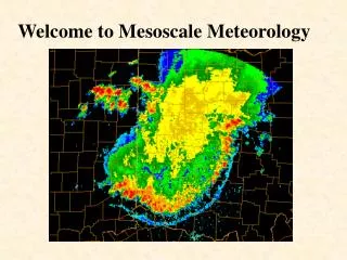
Welcome to Mesoscale Meteorology. Scale definitions - historical. Synoptic scale :. - derived from Greek “synoptikos” meaning general view of the whole. In meteorology has been accepted to imply “simultaneous”, since the “view of the whole” is

E N D
Scale definitions - historical Synoptic scale: - derived from Greek “synoptikos” meaning general view of the whole. In meteorology has been accepted to imply “simultaneous”, since the “view of the whole” is obtained by mapping observations made simultaneously at a number of locations. - the scales of fronts and cyclones studied first by Norwegian scientists. The “classic” definition of the synoptic scale was based on the space scales resolved by observations taken at European cities, which have a mean spacing of about 100 km. Weather systems having scales of hundreds of kilometers and time scales of a few days are generally accepted to be “synoptic scale” phenomena.
Scale definitions - historical Cumulus scale: • the scale of individual thunderstorms and cumulus cells. • This scale became the second important scale of • meteorological research when radars first began observing • weather systems after World War II. • -Spatial scale of about 1-50 km and time scale of a few minutes to • several hours.
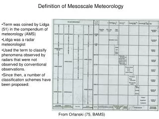
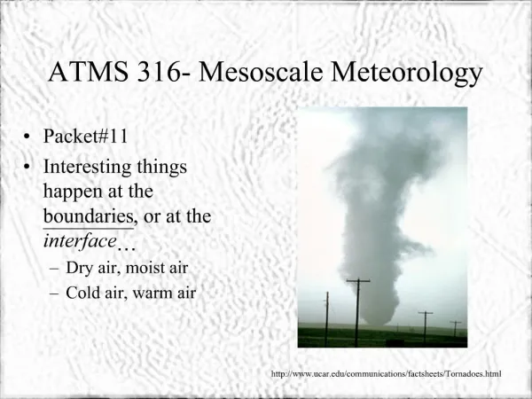
Scale definitions - historical Mesoscale: First coined by M. Lidga* (MIT radar meteorologist) in 1951 “It is anticipated that radar will provide useful information concerning the structure and behavior of that portion of the atmosphere which is not covered by either micro- or synoptic meteorological studies. We have already observed on with radar that precipitation formations which are undoubtedly of significance occur on a scale too gross to be observed from a single station, yet too small to appear even on sectional synoptic charts. Phenomena of this size might well be designatedmeso-meteorological.” *Ligda, M. G. H., 1951: Radar storm observations. In Compendium of Meteorology, AMS, Boston, 1265-1282
Scale definitions - historical Mesoscale: Concept expanded in paper by Tepper (1959) “…the emphasis on the larger scale motion and the deliberate disregard of the smaller scale motions has become well engrained among meteorologists.” He argued that motions smaller than macro-scale are not meteorologically insignificant or “meteorological noise”, but rather are vital to local forecasts. Tepper, M., 1959: Mesometeorology – the link between macro-scale atmospheric Motions and local weather. Bull. Amer. Meteor. Soc., 40, 56-72.
Scale definitions - modern There have been several papers that attempt to “define” mesoscale Orlanski, I, 1975: A rational subdivision of scales for atmospheric processes. BAMS, 56, 527-530 Fujita, T. T., 1981: Tornadoes and downbursts in the context of generalized planetary scales. J. Atmos. Sci., 38, 1512-1534. Fujita, T. T., 1986: Mesoscale classifications: their history and their application to forecasting. Chapter 2, Mesoscale Meteorology and Forecasting, pp. 18-35 Emanuel, K.A., 1986: Overview and definition of mesoscale meteorology. Chapter 1, Mesoscale Meteorology and Forecasting. pp 1-17. Thunis, P., and R. Bornstein, 1996: Hierarchy of Mesoscale Flow Assumptions and Equations. J. Atmos. Sci., 53, 380–397.
Orlanski (1975) proposed a scale definition based on the characteristic time and size of atmospheric phenomena This scale remains the most widely used terminology in meteorology because of its simplicity
Fujita (1981) and (1986) proposed a scale that was based on order-of-magnitude categories starting at the circumference of the earth 40000-4000 km Maso- 4000-400 km Maso- 400-40 km Meso- 40-4 km Meso- 4-0.4 km Miso- 400-40 m Miso- 40-4 m Moso- 4-0.4 m Moso- 40-4 cm Musu- 4-0.4 cm Musu- Fujita’s scale never caught on with the meteorological community
Emanuel (1986) viewpoint Scales have traditionally been assigned based on: observations observation networks theory Mesoscale meteorology involves: specific processes of energy transfer special events associated with instability or local forcing
Physical significance of scales of motion: Definition of system: Emanuel proposes defining a “system” as a rapidly evolving perturbation in a more slowly evolving larger circulation (e.g. below). (Can you think of other examples?)
Scales associated with atmospheric systems: Some scales are naturally defined by radiational processes (troposphere depth, diurnal cycle, N-S temperature gradient). Some scales may be related to the normal mode oscillations inherent in the atmosphere (gravity waves, Rossby waves) Some scales may be related to instabilities in the atmosphere (convective cells, jetstream circulations associated with interial instability) Some scales may be related to external forcing of flows (sea breeze, lake effect storms, mountain waves, valley flows)
Emanuel proposes a natural breakdown of phenomena into free (associated with instabilities) forced (circulations driven by boundaries). Factors that control convective instabilities operate below the mesoscale, although the resulting circulations, such as MCSs, are considered mesoscale. The Mesoscale Convective System is an example of convective instability, but on what scale? The Hurricane is an example of an air-sea interaction instability, but on what scale?
Consider the simplified frictionless equations of motion: We can write these in natural coordinates (see Holton, p. 57) as Force balance parallel to flow direction “s” Force balance normal (n) to flow direction “s” Force balance in vertical
PHYSICAL SIGNIFICANCE OF MESOSCALE Two major categories of force balances result: gravity vs. vertical PGF Hydrostatic Inertial (geostrophic) Coriolis vs. Horizontal PGF (inertial) Coriolis vs. Centrifugal force H. PGF vs. Centrifugal force (cyclostrophic) H. PGF vs. Centrifugal And Coriolis force (gradient)
Perturbations from balance For stable balance: Stability restores balance: perturbations initiate oscillations that result in waves For unstable balance: A growing disturbance results
Perturbations from Hydrostatic Balance Perturbations from stable balance lead to gravity (buoyancy) waves Horizontal phase speed Perturbations from unstable balance leads to convection
Perturbations from Inertial Balance Perturbations from stable balance lead to inertial (e.g. Rossby) waves Horizontal phase speed Perturbations from unstable balance leads to disturbances (e.g. baroclinic instability and cyclones)
In nature, both hydrostatic and inertial, stable and unstable balances exist and the flow is perturbed in numerous ways So what is the result?? Depends on which adjustment dominates…. We can estimate what the dominant adjustment will be from the ratio of the gravity wave speed to the inertial wave speed Rossby Radius of Deformation
What is the Rossby Radius of Deformation? Scale at which there is an equal inertial and gravity wave response The Rossby Radius is given by: In the middle latitudes: f ~ 10-4 s –1 H ~ 10 km (depth of disturbance) N ~ 1 10 –2 s –1 Rossby radius of deformation is about 1000 km
MESOSCALE METEOROLOGY Scale based on Physical Mechanisms Small scales (Lx << LR) - Tendency toward hydrostatic balance with gravity the dominant restoring force for perturbations. Large scales (Lx >> LR) - Tend toward geostrophic balance with the Coriolis force the dominant restoring force for perturbations.
Meso-g Scale 2 – 20 km (<< Rossby radius) Disturbances characterized by gravity (buoyancy) waves in stable conditions and convection in unstable conditions Coriolis effect generally negligible, although local inertial effects can arise to change the character of the disturbance
Tornadoes Supercells Valley flows Lake-effect convection
Meso-b Scale 20 – 200 km (Approaching Rossby radius) Gravity (buoyancy) waves govern system evolution Organized convection in unstable conditions Inertial oscillations important to wave dynamics (gravity-inertia waves) Inertial effects modify the organization of convection
Sea Breeze convection Mesoscale convective system Hurricane eyewall
Meso-a Scale 200 – 2000 km (> Rossby radius) Smaller circulations characterized by gravity-inertia response Larger circulations characterized by near geostrophic/gradient wind balance Ageostrophic circulations driven by disturbances in balanced flow
Mesoscale convective vortex Hurricane Fronts Jetstreaks
Meso a,b,g designations a convenience, but are neither firm boundaries nor clear discriminators of underlying dynamics Consider for example that: Changes in latitude alter the Coriolis effect Hurricane at 10°N vs 40°N Tropical squall line vs Mid-latitude squall line Coriolis is 0 at equator – equatorial disturbances are governed by gravity waves even at the global scale! Changes in the depth of a system alters the governing dynamics Sea breeze with convection vs. without Convective vs Stratiform region of MCS
Rotation induced by the system can shrink the Rossby radius altering the governing dynamics Mesocyclone with its gust fronts Contracting eyewall of a hurricane
Problems for mesoscale research: • Synoptic observation systems have horizontal resolutions of 50 km (or worse) and 1 hour at the surface and 400 km and 12 hours aloft and are clearly inadequate to capture all but the upper end of the meso-a. • The dynamics of mesoscale disturbances contain important non-balanced or transient features that propagate rapidly. • The systems are highly three-dimensional so that the vertical structure is equally important to the horizontal structure.
Problems for mesoscale research: • Mesoscale disturbances are more likely to be a hybrid of several dynamic entities interacting together to maintain the system. • Process Interaction is especially significant. Such processes include microphysical and radiative transfer interactions. • Scale Interactions and particularly interactions across the Rossby Radius of Deformation are basic to the mesoscale problem
Approaches to understanding mesoscale processes 1. Observations (advantages) Discovery: Mesoscale phenomena are discovered through observation (Models rarely if ever predict the existence of a phenomena until it is observed). Structure: The basic physical structure of phenomena can be described through analysis of observations Hypothesis: Hypotheses concerning the dynamic forcing thermodynamic processes, and microphysical processes are posed on the basis of observations. Validation: Observations serve as the benchmark for validating the quality of numerical model simulations of the phenomena.
Approaches to understanding mesoscale processes 1. Observations (disadvantages) Incomplete: Mesoscale phenomena are never observed adequately to determine their complete structure or underlying dynamics Dynamically inconsistent: Observations have errors that are large enough that the dynamics of mesoscale systems are difficult to retrieve. Rare: Focused field campaigns that cost millions of dollars are required to collect special data sets. These often yield a few high quality case studies.
Approaches to understanding mesoscale processes 2. Modeling (advantages) Comprehensive dataset: Understanding the dynamics of mesoscale phenomena requires a temporally and spatially complete, dynamically consistent data set, all of which a model provides. High resolution: Models can now simulate many mesoscale phenomena at high resolution. Dynamically consistent: If the model is consistent with the observations, then the model can be used (always with caution) to reveal the dynamics of the system.
Approach in understanding mesoscale processes 2. Models (disadvantage) Modeled processes inconsistent with true atmospheric behavior: Parameterizations within model (e.g. radiation, boundary layer forcing, diffusion, microphysical processes, convection) Can produce misleading, yet good looking solutions (worst case: right answer for wrong reason). Boundaries and initial conditions inconsistent with atmosphere structure and forcing: Poorly posed boundary conditions and initial conditions can render model solutions inadequate.
Approach in understanding mesoscale processes 3. Theory Explain basic phenomena in terms of analytical solution to governing equations. Advantage: Explanation is grounding in basic physical arguments. Provides foundation for understanding. Disadvantage: Can be wrong or misleading. Example: The Conditional Instability of the Second Kind (CISK) theory for tropical cyclone formation, taught for almost 40 years, did not incorporate air-sea interaction processes related to sea surface temperature and near surface wind speed.
OUR APPROACH IN THIS COURSE We will be reviewing key papers that present the most complete observations, high resolution revealing model simulations, and basic theory for mesoscale phenomena.