
Supply
E N D
Presentation Transcript
Supply MBA NCCU Managerial Economics Lecturer: Jack Wu
Case:DRAM Industry, 1996-98 • Prices falling sharply: • Fujitsu closed Durham, UK, factory but continued production at Gresham, OR • Texas Instruments sold Richardson TX, Italy, and Singapore plants to Micron • TI shut Midland, TX plant
Question • Question: explain differences in strategic decisions: • why did Fujitsu close Durham? • why did it continue with Gresham? • Question: Why did Micron buy some TI plants?
Business Response to Price Changes • If market price falls, should business reduce production or shut down? • Correct managerial decision depends on time horizon – which inputs can be adjusted. • Focus on short run, then later consider long run; • distinction between short/long run on supply side similar to that on demand side
Adjustment Time • short run: time horizon within which seller cannot adjust at least one input • long run: time horizon long enough for seller to adjust all inputs
Short-Run Cost Analyze total cost into two categories • fixed cost – do not vary with production scale • variable cost – does vary • marginal cost = increase in total cost for production of additional unit • average (unit) cost = total cost / production rate
Common Misconception • Capital expenditure = fixed cost • Labor = variable cost • Example: • US: workers employed “at will”. • Western Europe: strong worker protection laws • Japan: guaranteed lifetime employment • Current: temporary workers
Short-Run Total Cost total cost 8 variable cost 6 Cost (Thousand $) 4 2 fixed cost 0 2 4 6 8 Production rate (Thousand dozens a week)
DIMINISHING MARGINAL PRODUCT • Marginal product: increase in output from additional unit of input • Diminishing marginal product: marginal product reduces with each additional unit of input
SHORT-RUN MARGINAL, AVERAGE VARIABLE, AND AVERAGE COSTS diminishing marginal product causes marginal and average cost curves to rise 300 Cost (Cents per dozen) 250 200 marginal cost 150 average cost 100 average variable cost 50 0 2 4 6 8 Production rate (Thousand dozens a week)
MARGINAL REVENUE • Total revenue = price x sales quantity. • Marginal revenue: change in total revenue from selling additional unit • May be positive or negative • If price is fixed, then marginal revenue is equal to price
SHORT-RUN PROFIT, II total cost variable cost total revenue 4.793 loss = $1293 3.5 Cost/revenue (Thousand $) 0 1 5 9 Production rate (Thousand dozens a week)
Short-Run Decisions • Two key business decisions: • whether to continue in operation • scale of operation
Short-Run Production produce where marginal cost = price Cost/revenue (Cents per dozen) marginal cost average cost average variable cost 70 marginal revenue = price 5 break-even price Production rate (Thousand dozens a week)
Short Run Breakeven I produce if • total revenue >= variable cost, or • price >= average variable cost
Short Run Breakeven II • Sunk cost: cost that has been committed and cannot be avoided. • sunk costs should be ignored in making a current decision • assume, for competitive markets analysis, fixed cost = sunk cost • hence, a business should continue in production so long as its revenue covers variable cost (i.e. shut down if losses are greater than fixed cost) • or equivalently, so long as price covers average variable cost.
Short-Run supply curve • individual seller’s supply curve: that part of the marginal cost curve above minimum average variable cost; • minimum average variable cost -- short-run breakeven level.
Short-run individual supply: Input demand • Change in input price • shift in marginal cost • change in profit-maximing production
Long-Run Decisions • whether to enter/exit • price >= average cost • scale of operation • where marginal cost = price
Fujitsu • Durham, UK: long-run price < average cost (including cost of refitting) • Gresham, OR: average variable cost < short-run price < average cost
Why did Micron buy TI plants? • different views of long-run DRAM price • Micron could achieve greater scale economies • Why didn’t Micron buy all of TI’s plants? Possible explanation: • Micron Electronics bought TI plants -- Singapore, Italy, Richardson TX -- with lower average cost • TI closed plants with higher average cost -- Midland TX -- Micron didn’t wish to buy
Individual Supply • Graph of quantity that seller will supply at every possible price • follows marginal cost curve • slopes upward -- increasing marginal cost of production (or decreasing marginal return to inputs)
Supply Curve: Two Views • For every possible price, it shows the production/ delivery rate • For each unit of item, it shows the minimum price that the seller is willing to accept
Market Supply, I Graph of quantity that seller will supply at every possible price • horizontal sum of individual supply curves
Market Supply, II • lowest cost seller defines starting point • gradually, blends in higher-cost sellers • slopes upward
Long-Run Supply • long run -- freedom of entry and exit • if a business earns profits • attract new entrants • increase market supply • reduce market price • if business making loss, will exit
Long-Run Supply Curve slope of long-run supply • gentler than short-run supply • may be flat
Seller Surplus • Individual seller surplus = revenue a seller gets from a product - production cost • Market seller surplus = sum of individual seller surpluses
INDIVIDUAL SELLER SURPLUS individual seller surplus marginal cost c b 70 marginal revenue = price d d Cost/revenue (Cents per dozen) 43 a 0 1 5 Production rate (Thousand dozens a week)
Bulk Order • use bulk order to extract seller surplus • Sellers use package deals, two-part tariffs to extract buyer surplus; • buyer can apply symmetric concept -- how to get most out of seller; • use bulk purchasing to capture all seller surplus -- Speedy should offer Luna a lump sum equal to area 0abd plus $1 of seller surplus to supply a bulk order of 5000 dozen eggs
Profit/Price Variation: Lihir Gold IPO, Oct. 1995 • Projected profit in 1999: • $52m if gold price = $400 per ounce • $76m if gold price = $450 per ounce • Why would a 12.5% increase in gold price raise profit by 46%?
FORECASTING • Forecasting quantity supplied • Change in quantity supplied = price elasticity of supply x change in price