Download
1 / 15
160 likes | 180 Views
This project aims to improve field calculations by employing a more realistic model for the ATLAS solenoid, enhancing momentum accuracy in W mass measurements. Explore closed-loop model, field calculation corrections, helical model, and further work.

E N D
Realistic Model of the Solenoid Magnetic Field • Objectives • Closed-loop model • Field calculation corrections • Helical model • Realistic model • Conclusions + further work Paul S Miyagawa, Steve Snow University of Manchester
Objectives • A useful test of the Standard Model would be measurement of W mass with uncertainty of 25 MeV per lepton type per experiment. • Momentum scale will be dominant uncertainty in W mass measurement. • Momentum accuracy depends primarily on alignment and B-field. • Solenoid field mapping team targetting an accuracy of 0.05% on sagitta to ensure that B-field measurement is not the limiting factor on momentum accuracy. • Mapping machine will take measurements of the solenoid B-field. • Simulations of the machine performance have been based on a simple model of the B-field. • Want to test the performance with a more realistic model. • Realistic model seeks to improve on several aspects: • Calculating the field from a curved current path • Modelling the actual current path • Modelling the shape of the solenoid Mini-workshop on Magnetic Field Modelling
Closed-Loop Model • Previously, the solenoid was modelled as a series of closed circular loops of infinitely thin wires evenly spaced in z. • For calculating the field, each loop approximated as 800 straight-line segments, and Biot-Savart law applied to each segment. • Added in field due to magnetised iron (4% of total field). • Model is symmetric in and even in z. Mini-workshop on Magnetic Field Modelling
Field Calculation Corrections • We approximate the true current path, which is helical, with straight-line segments whose end points lie on the true path. • This leads to two types of error: Inscribed polygon error • If a circle is replaced by an inscribed polygon, the average radius of the polygon is less than the radius of the circle. • This effect can be corrected by increasing the radius by 2/3 of S where S is the sagitta between the arc and the chord. Line segment integration error • The natural approximation is to use the midpoint of the segment to calculate r between the segment and the measurement point. • This leads to an error because r is different for each point on the line. This error is more significant than the inscribed polygon error. • A correction factor can be added to the magnitude of the field: Mini-workshop on Magnetic Field Modelling
Field Calculation Corrections z = 0, r = 0 z = 1, r = 0 z = 0, r = 0.8 z = 1, r = 0.8 Mini-workshop on Magnetic Field Modelling 100 steps most likely sufficient, but we use 200 to be safe.
Helical Model • First step towards a realistic model is to replace the series of closed loops with a helical coil. • The current starts at (0,R,hz), winds in anti-clockwise direction, and terminates at (0,R,-hz). Note that this does not form a closed path. • The overall dimensions of the coil are the same as for the closed-loop model. • Model is neither symmetric in nor even in z. • Main differences with closed-loop model are at the ends of the coil due to difficulty in lining up the ends. Mini-workshop on Magnetic Field Modelling
Realistic Model • The ATLAS solenoid consists primarily of four main coil sections. • The last loop from each section is welded to the first loop of the next section to form a single coil. • At end A, an extra cable is welded to the last loop, and the two cables are routed up through the services chimney. • At end C, an extra cable is welded to the last loop. The two cables form the return current conductor, which is routed along the cryostat surface to end A and up into the chimney. • Cables in the chimney are magnetically shielded. • The realistic model models the current through these main components. Mini-workshop on Magnetic Field Modelling
Main Coil Sections • From end A to end C, the four coil sections are labelled H-A, F-A, F-C and H-C. • Each section is modelled as a shorter version of the helical coil with its own length and number of loops. • The winding direction gives the B-field in the +z direction. • The loops at either end of each section are treated in the welds, so are not included in the main sections. Mini-workshop on Magnetic Field Modelling
Internal Welds • Physically, the last loop from one section lies parallel to the first loop of the next section. These two loops are welded together along their entire length so that electrically they are one loop. • Two models of these welds can be used: • The physical representationuses two loops running in parallel. The current gradually transfers from the first loop to the second. • The electrical representation uses a single loop of double pitch. This loop carries the full current over its entire length. • Model of internal weld has negligible effect on B-field. Mini-workshop on Magnetic Field Modelling
End Welds • At each end of the solenoid, the extra cable is welded to the main cable over a 30-cm portion. This is actually 90°, so this will have to be corrected. The current starts entirely in the main cable, and 20% is transferred to the extra cable by the end of this portion. • The two cables follow the curvature of the solenoid over 4.5°, but are electrically isolated from each other. They carry the current in the ratio 80:20. • The two cables then curve away from the solenoid until they are tangent to the chimney angle (11.25° from vertical). The radius of curvature is 165 mm. As the cables are still electrically isolated, they carry the current in the same 80:20 ratio. End A End C Mini-workshop on Magnetic Field Modelling
Return Current Conductor • The return current conductor consists of the two cables from the end C weld running flat along the cryostat surface. The extra cable rests on top of the main cable. • The cables are electrically isolated, so they carry the current in ratio 80:20. • In the realistic model, the cables connect to the cables from the end A weld so as to form a closed current path for the entire solenoid. Mini-workshop on Magnetic Field Modelling
The dimensions given are for a warm coil in quiescent conditions. The real coil will be deformed: Shrinkage due to cool down. This is modelled as an overall scale reduction of 0.41%. Bending due to field excitation. This is modelled as the radius r being a parabolic function of z. At the centre, Δr = 0.90 mm; at the coil ends, Δr = 0.38 mm, Δz = 1.09 mm. Shape Deformations Mini-workshop on Magnetic Field Modelling
Field from Realistic Model Mini-workshop on Magnetic Field Modelling
Conclusions • Developed realistic model of the solenoid B-field which makes several improvements over the simple closed-loop model. • Corrections made for errors which arise from approximating curved current paths with straight-line segments: • inscribed polygon error • line segment integration error • Modelled the actual current path: • four main coil sections • welds between main sections • welds at end of solenoid • return current conductor • Modelled real shape of solenoid: • shrinkage due to cool down • bending due to field excitation • Made comparisons with previous model: • Most adjustments to Bz and Br components are O(10 gauss). • Greatest adjustments are at boundaries (coil ends, weld regions). • Return coil has greatest effect on Bφ component. Mini-workshop on Magnetic Field Modelling
Further Work • Investigate further refinements of realistic model: • Correct the weld portion of the end welds. • Current flow through cable cross-section (2×6 array of wires). • Simulate performance of field mapping machine and fitting routines using B-field from realistic model. Mini-workshop on Magnetic Field Modelling