Results of the ATLAS Solenoid Magnetic Field Map
Results of the ATLAS Solenoid Magnetic Field Map. CERN mapping project team Martin Aleksa, Felix Bergsma, Laurent Chevalier, Pierre-Ange Giudici, Antoine Kehrli, Marcello Losasso, Xavier Pons, Heidi Sandaker Map fitting by John Hart (RAL) Paul S Miyagawa , Steve Snow (Manchester). Outline.


Results of the ATLAS Solenoid Magnetic Field Map
E N D
Presentation Transcript
Results of the ATLASSolenoid Magnetic Field Map CERN mapping project team Martin Aleksa, Felix Bergsma, Laurent Chevalier, Pierre-Ange Giudici, Antoine Kehrli, Marcello Losasso, Xavier Pons, Heidi Sandaker Map fitting by John Hart (RAL) Paul S Miyagawa, Steve Snow (Manchester)
Outline • Overview of mapping campaign • Corrections to data • Geometrical fit results • Geometrical + Maxwell fit results • Systematic errors • Conclusions EPS HEP 2007, Manchester, 20 July 2007
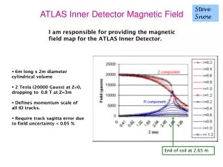
ATLAS Experiment • LHC will produce proton-proton collisions: • cms energy 14 TeV • 25 ns bunch spacing • 1.1×10¹¹ protons/bunch • design luminosity 1034 cm-2s-1 • ATLAS is a general-purpose detector: • diameter 25 m, length 46 m • overall mass 7000 tonnes • ATLAS solenoid provides 2 T field for Inner Detector • length 5.3 m, diameter 1.25 m, 1159 turns • operated at 7730 A EPS HEP 2007, Manchester, 20 July 2007
Overview of the task • Mapping 6m long x 2m diameter cylindrical volume • 2 Tesla (20000 Gauss) at Z=0, dropping to 0.8 T at Z=3m • Require track sagitta error due to field uncertainty < 0.05% • Motivated by targets on uncertainty for measurement of W mass EPS HEP 2007, Manchester, 20 July 2007
The field mapping machine Cards each hold 3 orthogonal sensors Pneumatic motors with optical encoders. Move and measure in Z and φ. EPS HEP 2007, Manchester, 20 July 2007 4 arms in windmill. Each arm equipped with 12 Hall cards 4 fixed NMR probes at Z=0
Data sets recorded • Data taken at four different solenoid currents • Nominal current (7730 A) gives 2 T at centre • Low current (5000 A) gives 1.3 T and is used with low-field probe calibration • Fine phi scans used to measure the (tiny) perturbation of the field by the mapping machine • Total data collected ~0.75M • Statistical errors will be negligible EPS HEP 2007, Manchester, 20 July 2007
Corrections to data Geometrical effects • Plenty of survey data taken before and after mapping campaign • Positions of individual Hall sensors can be determined to ~0.2 mm accuracy • Mapping machine skew recorded in data • Carriage tilts determined from data Probe calibrations • Response of Hall sensors calibrated as function of field strength, field orientation and temperature using test stands at CERN and Grenoble • Low-field calibration (up to 1.4 T) has expected accuracy of ~2 G, 2 mrad • High-field calibration (up to 2.5 T) has expected accuracy of ~10 G, 2 mrad • NMR probes intrinsically accurate to 0.1 G • Absolute scale of high-field Hall calibration improved using low-field Hall calibration and NMR values • Relative Hall probe normalisations and alignments determined from data Other effects • Effects of magnetic components of mapping machine corrected using magnetic dipoles EPS HEP 2007, Manchester, 20 July 2007
Fit quality measures • We fit the map data to field models which obey Maxwell’s equations • The volume covered has no currents and has effects of magnetic materials removed • Maxwell’s equations become • Our fit uses Minuit to minimise • Our aim is to know the track sagitta, which is proportional to (cr and cz are direction cosines) • Our fit quality is defined to be δS/S where EPS HEP 2007, Manchester, 20 July 2007
Geometrical fit • 96% of the field is directly due to the solenoid current • We use a detailed model of the conductor geometry and integrate Biot-Savart law using the known current • 7 free parameters • Scale factor and aspect ratio (length/diameter) of conductor model • Position and orientation of conductor model relative to IWV • 4% of field is due to magnetised iron (TileCal, girders, shielding discs etc) • Parametrised using 4 free parameters of Fourier-Bessel series with length scale=2.5m Conductor geometry determined by surveys of solenoid as built except weld thickness, which was determined from data as 1.9×pitch EPS HEP 2007, Manchester, 20 July 2007
Results from geometrical fit BZ BR Bφ 20 G 20 G 20 G 20 G 20 G 20 G 20 G 40 G 40 G EPS HEP 2007, Manchester, 20 July 2007
Full fit (geometrical + Maxwell) • A few features remain in the residuals from the geometrical fit • Ripples for |Z|<2m believed to be due to variations in the coil winding density • Bigger features at |Z|>2m believed to arise from the coil cross-section not being perfectly circular • These effects are more pronounced at the ends of the solenoid • These features cannot be determined accurately enough to be included in the geometrical model • However, they are real fields which should obey Maxwell’s equations • We apply a general Maxwell fit to the residuals to account for these features EPS HEP 2007, Manchester, 20 July 2007
General Maxwell fit • General fit able to describe any field obeying Maxwell’s equations. • Uses only the field measurements on the surface of a bounding cylinder, including the ends. • Parameterisation proceeds in three stages: • Bz on the cylindrical surface is fitted as Fourier series, giving terms with φ variation of form cos(nφ+α), with radial variation In(κr) (modified Bessel function). • Bzmeas – Bz(1) on the cylinder ends is fitted as a series of Bessel functions, Jn(λjr) where the λj are chosen so the terms vanish for r = rcyl. The z-dependence is of form cosh(μz) or sinh(μz). • The multipole terms are calculated from the measurements of Bron the cylindrical surface, averaged over z, after subtraction of the contribution to Br from the terms above. (The only relevant terms in Bz are those that are odd in z.) EPS HEP 2007, Manchester, 20 July 2007
Results from full fit I BZ BR Bφ 20 G 20 G 20 G 20 G 20 G 20 G 20 G 40 G 40 G EPS HEP 2007, Manchester, 20 July 2007
Results from full fit II • All fit parameters (length scale, position, etc) consistent with expected results • With full fit, residuals of all probes reduced significantly • Recall that Maxwell fit is made using outermost probes only • Fact that the fit matches inner probes as well shows strong evidence that the difference between data and geometrical model is a real field • With geometrical fit alone, rms of relative sagitta error δS/S already within target of 5×10⁻⁴ • Adding Maxwell fit improves δS/S, especially at high η EPS HEP 2007, Manchester, 20 July 2007
Systematic errors • Uncertainty in overall scale • Comparison between Hall and NMR probes • Weld thickness, which influences the Hall-NMR comparison • Overall scale error 2.1×10⁻⁴ • Uncertainty in shape of field • Dominant factor is 0.2 mrad uncertainty in orientation of the mapping machine relative to ATLAS physics coordinates • Overall shape error 5.9×10⁻⁴ • Total uncertainty varies from 2–11 ×10-4 • Dominated by scale error at low η, shape error at high η EPS HEP 2007, Manchester, 20 July 2007
Conclusions • The ATLAS solenoid field mapping team recorded lots of high quality data during a successful field mapping campaign • All possible corrections from surveys, probe calibrations and probe alignments have been applied to the data • We have determined a fit function satisfying Maxwell’s equations which matches each component of the data to within 4 Gauss rms • Using this fit, the relative sagitta error ranges from 2–11 ×10-4 • At high rapidity, the systematic errors are dominated by a 0.2 mrad uncertainty in the direction of the field axis relative to the ATLAS physics coordinate system EPS HEP 2007, Manchester, 20 July 2007
Survey of mapping machine in Building 164 Radial positions of Hall cards Z separation between arms Z thickness of arms Survey in situ before and after mapping Rotation centre and axis of each arm Position of Z encoder zero Positions of NMR probes Survey of ID rails Gradient wrt Inner Warm Vessel coordinates Survey of a sample of 9 Hall cards Offsets of BZ, BR, Bf sensors from nominal survey point on card Sensor positions known with typical accuracy of 0.2 mm Surveys EPS HEP 2007, Manchester, 20 July 2007
Hall sensors Response measured at several field strengths, temperatures and orientations (θ,φ) Hall voltage decomposed as spherical harmonics for (θ,φ) and Chebyshev polynomials for |B|,T Low-field calibration (up to 1.4 T): expected accuracy ~2 G, 2 mrad High-field calibration (up to 2.5 T): expected accuracy ~10 G, 2 mrad NMR probes No additional calibration needed (done by whoever measured Gp = 42.57608 MHz/T) Compare proton resonance frequency with reference oscillator Intrinsically accurate to 0.1 G Probe calibrations EPS HEP 2007, Manchester, 20 July 2007
Probe normalisation and alignment • Exploited the mathematics of Maxwell’s equations to determine relative probe normalisations and alignments • BZ normalisation: • Uses the fact that each probe scans the field on the surface of a cylinder • BZ at centre determined for each probe • All probes were then normalised to the average of these values • Probe alignment: • Uses curl B = 0 and • Integrate • Tilt angles Aij of probe were determined from a least squares fit • The third alignment angle comes from div B = 0 EPS HEP 2007, Manchester, 20 July 2007
Carriage tilts • Another analysis which exploited mathematics of Maxwell • Bx and By on the z-axis evaluated from average over φ for probes near centre of solenoid • Plots of Bx,By versus Z of carriage show evidence that entire carriage is tilting • Degree of tilt can be calculated by integrating to find expected Bx,By value • Jagged structure of tilts suggest that machine is going over bumps on the rail of ~0.1 mm EPS HEP 2007, Manchester, 20 July 2007
Absolute scale of high-field Hall calibration (10 G) is greatest uncertainty Can be improved using low-field Hall calibration (2 G) and NMR value (0.1 G) Low-field Hall values and NMR values are equal for 5000 A data Low-field Hall values are considered accurate in low-field region Discrepancy between low- and high-field Hall values in low-field region Discrepancy between high-field Hall values (derived from field fits) and NMR value in high-field region This discrepancy lines up with the discrepancy from low-field region Alternative high-field Hall values from extrapolation give estimate of systematic error Absolute Hall scale EPS HEP 2007, Manchester, 20 July 2007
Magnetic machine components • Perturbation of the magnetic field by the mapping machine was not anticipated • Some spikes in the data were clearly attributed to components of the mapping machine • A dipole was subtracted at each component position with field strength chosen to make residuals look smooth EPS HEP 2007, Manchester, 20 July 2007