Download

1 / 54
540 likes | 673 Views
Business Cycles and the Dynamics of GDP. Chap. 27. Global Financial Crisis. Why did output fall globally, why so much, and why has it lasted so long?. Statistics OECD. HK Contraction and Recovery. Hong Kong Census & Statistics. Hong Kong Census & Statistics. Two Impressions.

E N D
Global Financial Crisis • Why did output fall globally, why so much, and why has it lasted so long? Statistics OECD
HK Contraction and Recovery Hong Kong Census & Statistics
Two Impressions • GDP Volume is growing over time. • Growth is variable. Sometimes fast, sometimes flat, sometimes negative. • Decompose the series into two parts which capture each of these phenomena. • Potential GDP • Output Gap
GDP is output per worker times number of workers. Labor Productivity GDP and Productivity
Unemployment Rates • The population resides in 1 of 3 categories • Not in the Labor Force: Not working and not actively seeking work • Labor Force • Employed: Currently working. • Unemployed: Not working but seeking work. Unemployment Rate
Natural Rate of Unemployment • Always people losing or leaving jobs and looking for new ones. Always people joining the labor force. • In natural state of labor market, people looking for jobs will match the number of people who find jobs. • uN = Natural Rate: Rate at which there is neither excess demand nor supply in labor market. (mostly stable).
Potential Employment and Output • Potential employment is the level of employment when unemployment equals the natural rate. • Potential output is GDP when employment equals potential employment
Hong Kong Census & Statistics HK GDP vs. Estimate of HK Potential GDP
Recessions and Expansions • The path of the economy is often divided into periods called recessions and periods caused expansions. • No precise definition of “recession” or “expansion” exists, sometimes as consecutive quarters of growth. • Business cycles are defined by the Output Gap, • Sometimes the period from peak of the output gap to the trough is a recession and the period when the output gap is increasing is an expansion. US Business Cycle Dates
Business Cycles Focus on explaining fluctuations in real GDP, Y, and the GDP Deflator, P. Framework reminiscent of the supply and demand model.
Two Aspects of Potential Output • Potential Output is unrelated to the price level but is determined by capital infrastructure, efficiency of labor markets, population, technological know-how. • Output increases above potential only if unemployment falls below natural level; • if unemployment rises above natural level, output will be below potential.
Potential output and labor market. • Potential output can be viewed as a level consistent with equilibrium in labor market. • Wages hit a level so workers want to work as many hours as firms want to hire. • When output is above potential output, low unemployment and the search for workers will push up wages. • When output is below potential, high unemployment and the surplus of workers will push down wages.
Potential Output YP P Unemployment above natural rate Unemployment below natural rate Upward Pressure on Wages Downward Pressure on Wages Y
Why does SRAS Slope Up?Take wages as given in Short Run • Money wages paid to workers adjust dynamically over time through negotiation. • At a given wage, a rise in the price level reduces the cost of labor relative to value of goods produced making hiring labor to produce goods more attractive. • At a given wage rate, higher prices induce higher production → in the short run, supply is positively associated with output.
Short Run Aggregate Supply Curve YP SRAS P Y
1. Shift in Potential Output • Advance in Technology Frontier, PP& E, or expansion in potential labor force (population, demographics). • Shifts SRAS w/ potential output. 2. Shifts in SRAS • When dollar cost of labor (or prices of energy) shift, changes in costs are passed on into prices. • Wages and other cost shifters shift SRAS at a given level potential output.
1. Expansion in Output Potential SRAS' YP ' YP SRAS P Y Normal for technological progress to increase potential output.
2. Increase in Wages SRAS' P YP SRAS Y
Expenditure: C + I + G + NX Prices and Spending • Wealth Effect – Real value of liquid/monetary assets rises as prices fall. This adds to wealth of households stimulating consumption. • Competitiveness Effect – Holding exchange rate constant, a lower price level makes domestic exports more attractive and foreign imports less stimulating net exports. For now, hold interest rate and exchange rate constant.
Aggregate Demand Curve P AD Y
Equilibrium • Equilibrium in the competitive market occurs when the price is set at a level (P*) such that the amount that consumers want to buy is equal to the amount that sellers want to sell (Y*). Excess SupplyIf P were above equilibrium, sellers would want to sell more goods than buyers would want to buy. Competition between sellers would force prices down. Excess DemandIf P were below equilibrium, customers would want to buy more goods than people would want to sell. Competition between buyers would force prices up.
Equilibrium GDP and Price Level P SRAS P* AD Y Y*
Output below potential: Recessionary Gap. P YP SRAS 1 P* AD GAP Y Y*
Output above potential: Inflationary Gap. YP SRAS P 2 P* AD GAP Y Y*
Self Correction Process • Business cycles have a natural end. • In short run, Y* may be greater than or less than potential output. However, in that case surplus or shortage of workers in labor markets will be putting downward or upward pressure on wages. • Pressure on wage costs will shift the supply curve until equilibrium output is equal to potential output.
AS1 YP P AS AS2 1 W↓ W↑ 2 AD Y Movement to Long Term Equilibrium
Cyclical Fluctuations • Period-by-period, different important events will impact the economy. We will think of these events as primarily driving the demand side of the economy (shifting the AD curve) or primarily driving the supply side (shifting the supply side). • The strength of these will determine the correspondence between movements in output and inflation.
Demand side shocks cause output and prices to move together. P SRAS P* 1 P** 2 AD1 AD2 Y Y** Y*
Output below potential. Downward pressure on wages. Cost of production falls and AS shifts down YP SRAS P SRAS2 1 2 As costs fall, competitive prices fall, there is a movement along the AD curve. 3 P*** Wages fall AD2 Y Y***
Wages will keep falling until the surplus of labor is absorbed – when prices fall enough that demand reaches potential output P SRAS2 SRAS3 3 Wages fall 4 AD2 Y YP
AS-AD and Expected inflation • Potential GDP generally increases at a consistent rate. • On average, aggregate quantity of liquid assets tends to increase faster than potential GDP. • Workers wages will tend to rise to match increases in the cost of living. • AD does not always rise evenly with GDP.
Dynamic AS-AD Model: Ideal YPt+1 YtP SRASt+1 P SRASt Demand expansion matches supply expansion P*t+1 Average Inflation Pt* ADt+1 ADt Y Yt* Y*t+1 Ch. 29, 711-712
Dynamic AS-AD Model: Recession, Inflation Deceleration ASt+1 YPt+1 YtP ASt P Demand expands slower than expected P*t+1 Expected Inflation Actual Inflation Pt* Inflation rises less than usual ADt+1 ADt Negative Output Gap Gap Y Yt* Y*t+1
Dynamic AS-AD Model: Inflation Acceleration Inflation rises more than usual YPt+1 YtP P ASt+1 ASt Demand expands faster than expected P*t+1 Actual Inflation Pt* Expected Inflation ADt+1 ADt Positive Output Gap Gap Y Yt* Y*t+1
Elements • Global Imbalances – Savings Glut • Real Estate Bubbles – Fueled by optimism and low global interest rates. • Precarious Financial Systems in Some Countries: Large holdings of real estate debt financed by financial institutions with high leverage. • Beginning in 2007, a series of failures or nationalizations of banking system.
Uncertainty About Investment, Decline in Wealth, Restrictions on Borrowing SLF SLFW’ r DLFW DLFW' rW rWW LF LFW