Branchwidth via Integer Programming
Explore the concept of branchwidth and Graph Minors Theorem in graph theory, with applications in solving NP-complete problems and constructing branch decompositions. Learn about Wagner's Theorem, well-quasi-ordering, and optimal branch decomposition algorithms.

Branchwidth via Integer Programming
E N D
Presentation Transcript
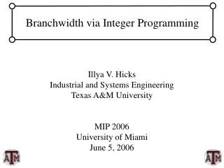
Branchwidth via Integer Programming Illya V. Hicks Industrial and Systems Engineering Texas A&M University MIP 2006 University of Miami June 5, 2006
Menu: 4-course meal • Background, Definitions & Relevant Literature • Branchwidth of Graphic Matroids • Integer Programming Formulation for Branchwidth • Conclusions & Future Work
Wagner’s Theorem Contracting e e A graph H is a minor of G if H can be obtained from a subgraph of G by contracting edges. Wagner’s Theorem: A graph G is planar if and only if G contains no minor of K5 or K3,3. K5 K3,3
Other surfaces • Erdös (1930’s) • posed the question of whether the list of minor-minimal graphs not embeddable in a given surface is finite. • Archdeacon (1980) and Glover, Huneke and Wang (1979) • proved that there are 35 minor-minimal non-projective planar graphs. • Archdeacon and Huneke (1981) • proved the list is finite for non-orientable surfaces. • Robertson and Seymour (1988) GMT • proved the list is finite for any surface.
Well-quasi-ordering and the Graph Minors Theorem • A class with a reflexive and transitive relation is a called a quasi-order. • A quasi-order, (Q, ), is well-quasi-ordered if for every countable sequence q1, q2, … of members of Q there exist 1 i < j such that qi qj. • Graph Minors Theorem: The “minor” quasi-order is well-quasi-ordered. • Example: One quasi-order that is not well-quasi-ordered is the “subgraph” quasi-order.
Branch Decompositions (Robertson and Seymour 1991) Let G be a graph. Let T be a tree with |E(G)| leaves where every non-leaf node has degree 3. Let be a bijection from the edges of G to the leaves of T. The pair (T, ) is called a branch decomposition of G. 2 G (T,) 0 1 0 3 2 4 3 1 4
e Branchwidth An edge of T, say e, partitions the edges of G into two subsets Aeand Be. The middle set of e, denoted as mid(e) or mid(Ae, Be), is the set of nodes of G that touch edges in Aeand edges in Be. The widthof (T,) is the maximum cardinality of any middle set of T. The branchwidth, (G),is the minimum width of any branch decomposition of G. A branch decomposition of G is optimal if its width is equal to (G). G 2 0 1 (T,) 0 3 2 4 3 1 4
2 3 7 8 0 a b {a, e, f} {f, g, h} 4 2 3 e f 6 10 5 1 {a, d, f, g} 7 6 5 11 8 g h {a, b, f} {a, c, g} 9 10 c d 0 4 1 9 11 Example Graph
Motivation • Arnborg, Lagergren and Seese (1991), based upon the work of Courcelle (1990), showed that many NP-complete problems modeled on graphs with bounded branchwidth can be solved in polynomial time using a branch decomposition based algorithm on the graph. • NP-complete problems modeled on graphs: • Minimum Fill-in • Traveling Salesman Problem • General Minor Containment • Constructing Branch Decompositions • Branch decomposition based algorithms
Constructing Branch Decompositions • Finding optimal or near-optimal branch decompositions is essential to the overall success of branch decomposition based algorithms because these algorithms are exponential in the width of the given branch decomposition. Times for Euclidean Steiner Tree Problem provided by Bill Cook
Phylogenetic trees 5,0 3,0 S1 100110 S2 001000 S3 110000 S4 110111 S5 001110 1,1 2,1 4,0 S3 S2 6,0 S1 2,0 6,1 4,1 S4 3,1 1,0 Column x Number y x,y 5,1 S5
Phylogenetic Trees S3 S1 S2 6 6 6 7 6 6 5 S4 S5
Constructing Branch Decompositions • Robertson and Seymour (1995) • given integer k and graph G,finds a branch decomposition with width 3k for some subgraph H of G such that either H = G or (H) ≥ k . • Bodlaender and Thilikos (1999) • computes branch decomposition for graphs with (H) ≤ 3 • Kloks, Kratochvil, Muller (1999) • Polynomial-time algorithm for the branchwidth of interval graphs • Hicks (2005) • branch decomposition based algorithm to construct optimal branch decompositions
Planar Branch Decompositions • Seymour and Thomas (1993) • polynomial time algorithm to compute the branchwidth and an optimal branch decomposition for planar graphs • Tamaki (2003) • Linear-time heuristic for near-optimal branch decompositions of planar graphs • Hicks (2005, 2005) • practical implementation of Seymour and Thomas algorithm • Gu and Tamaki (2005) • O(n3) algorithm for an optimal branch decomposition of a planar graph
Branchwidth Heuristics • Cook and Seymour (1994) • Finds separations using spectral graph theory • Diameter Method [Hicks 2002] • Finds separations such that nodes that are far apart are in different sets • Hybrid Method [Hicks 2002] • Uses the Cook and Seymour heuristic for the initial separation but the diameter method for subsequent separations.
Branch Decomposition Based Algorithms • Robertson and Seymour (1995) • theoretical algorithm for testing graph minor containment • Cook and Seymour (2003) • practical algorithm for solving TSP • Fomin and Thilikos (2003) • Theoretical algorithm for dominating set on planar graphs using branch decompositions • Fomin and Thilikos (2004) • Branchwidth of a planar graph is at most sqrt(4.5n) • Hicks (2004) • practical algorithm for testing graph minor containment • Hicks (2005) • practical algorithm for computing optimal branch decompositions
Menu: 4-course meal • Background, Definitions & Relevant Literature • Branchwidth of Graphic Matroids* • Integer Programming Formulation for Branchwidth • Conclusions & Future Work *Joint work with Nolan McMurray
Matroids • Let S be a finite set and I be a family of subsets of S, called independent sets. • M = (S, I) is called a matroid if the following axioms are satisfied • I • if J’ J I, then J’ I • for every A S, every maximal independent subset of A has the same cardinality, rank (A)
Matroid Examples: Cycle Matroids • Let G = (V, E) be a graph and let S = E • I = {J S: J is a forest of G} • a matroid is called graphicif it is the cycle matroid for some graph • denoted M(G)
Branch Decompositions Let M be a matroid. Let T be a tree with |S(M)| leaves where every non-leaf node has degree 3. Let be a bijection from the elements of S(M) to the leaves of T. The pair (T, ) is called a branch decomposition of M. 2 (T,) 0 1 0 3 2 G 4 3 1 4
Separations for Matroids • A separationof a matroid M(S, I)is a pair (A, B) of complementary subsets of S(M). • The order of the separation (A, B), denoted (M, A, B), is defined to be the following: • (A) + (B) - (M) +1, if A B • 0 , else
e Branchwidth An edge of T, say e, partitions the edges of S(M) into two subsets Aeand Be. The orderof e, denoted as order(e),is equal to (M,Ae,Be). The widthof (T,) is the maximum order of any edge of T. The branchwidth, M(M),is the minimum width of any branch decomposition of M. A branch decomposition of M is optimal if its width is equal to M(M). G 2 0 1 (T,) 0 3 2 4 3 1 4
f g 2 2 e d 2 3 3 f d 2 g 3 = 4 + 2– 4 + 1 e 2 c a b c 3 Euclidean Representation 2 2 a b Fano Matroid and its Optimal Branch Decomposition
Branchwidth of Matroids • Dharmatilake (1996) • Introduced branchwidth and tangles of matroids • Geelen et al. (2002) • matroid analogue of GMT • Hall et al. (2002) • Studied matroids of branchwidth 3 • Hliněný (2002) • excluded minors of matroids with branchwidth 3
Branchwidth of Matroids • Geelen, Gerards, Robertson, & Whittle (2003) • bounded size of excluded minors of matroid with branchwidth k • graphic matroid conjecture • Hicks and McMurray (2005) • The branchwidth of a graph is equal to the branchwidth of the graph’s cycle matroid if the graph has a cycle of length at least two • Mazoit and Thomasse (2005)
Matroid Tangles (Geelen et al. 2003) • A tanglein M(S, I) of order k is the set T corresponding to separations of M, each of order < k such that: MT1: For each separation (A, B) of M of order < k, one of A or B is an element of T. MT2: If A T and a separation (C,D) of order < k such that C A then C T. MT3:If e S(M), then e T. MT4: If (A1, B1), (A2, B2), (A3, B3) are separations of such that A1, A2, and A3partition S(M) then not all of A1, A2, and A3can be members ofT .
Matroid Tangles • The tangle numberof M, (M),is the maximum order of any tangle of M. • Theorem [Geelen et al. 2003] Let M be a matroid. If a tangle exists for M, then (M) = (M) . • If |S(M) | ≤ 3 or there exists a an element eS(M) such that (M, e, S(M) \e) ≥ k, then M has no tangle of order k.
Separations and Tangles of Graphs • A separationof a graph G is a pair (G1, G2) of subgraphs of G with G1 G2 = (V(G1) V(G2), E(G1) E(G2)) = G and E(G1) E(G2) = . • A tanglein G of order k is the set T corresponding to a set separations of G, each of order < k such that: T1 For each separation (A, B) of G of order < k, either A or B is an element of T. T2 If A1, A2, A3 T, then A1 A2 A3 G. T3 If A T, then V(A) V(G). • The tangle numberof G, (G),is the maximum order of any tangle of G.
a b c d Tangle of Order 3 for K4 T ={ (, G), (a, G), (b, G), (c, G), (d, G), ({a,b}, G), ({a,c}, G), ({a,d}, G), ({b,c}, G), ({b,d}, G), ({c,d}, G), (G[a,b], G\ab), (G[a,c], G\ac), (G[a,d], G\ad), (G[b,c], G\bc), (G[b,d], G\bd), (G[c,d], G\cd)}
Graph Tangles and Branchwidth • Theorem (Robertson and Seymour 1991): For any loopless graph G such that E(G) , max((G), 2) = (G). • Tangles can be used to prove lower bounds for branchwidth.
Cycle Matroid and Graph Separations (M, A, B) = |V(A)| – (A) + |V(B)| – (B) – |V(G)| + (G) + 1 = |V(A) V(B)| – (A) – (B) + (G) + 1
Main Theorem (Hicks and McMurray 2005) • Lemma: Let G be a connected graph with (G) ≥ 3 and let TG be a tangle for G of order k ≥ 3. Let TM(G) denote the set of separations of M(G) with order < k such that ATM(G) if for every component H of G[A], there exists C TG such that E(H) E(C). Then TM(G) is a tangle of M(G) of order k. • Main theorem: Let G be a graph with a cycle of at least 2 then (G) = (M(G))
Graphic Matroids and Planar Graphs • Given matroid M(S, I) then M*(S, I*) is called the dual of M if J I then S\J I*. • Theorem [Whitney 1933]: A graph is G is planar if and only if M*(G) is graphic. • Corrollary: Let G be a graph with a cycle of length at least two and let G* be its planar dual then (G) = (G*).
2 3 7 8 a b 0 4 2 6 10 e f 3 1 5 7 6 8 g a h 9 10 5 11 c d 0* 5* 1* 11* b c 4* 7* 3* 2* d 10* 0 4 1 9 11 6* 8* e f 9* Planar Graphs and their Duals • Theorem (RS 1994, Hicks 2000): Let G be a loopless planar graph and G*be the corresponding dual and loopless. Then β(G) = β(G*).
Menu: 4-course meal • Background, Definitions & Relevant Literature • Branchwidth of Graphic Matroids • Integer Programming Formulation for Branchwidth* • Conclusions & Future Work *Joint work with Elif Kotologlu and J. Cole Smith
Integer Programming Formulation for Branchwidth • Steiner tree packing problem • IP formulation • Relevant Cuts • Difficulties with Formulation • Preliminary Results
Steiner Tree Packing • Given a graph G = (V, E) with edge capacities ce for all eE and a list of terminal sets T ={T1, …, TN}, find Steiner trees S1, …, SN for each terminal set such that each edge eE is at most ce of the Steiner trees.
Steiner node terminal The load is 2 for this edge Steiner Tree Packing 0 4 3 1 2 T1={0,1,2} T2={2,3,4}
The Concept Objective: minimize maximum load M: nodes corresponding to the edges of G N:Steiner nodes e A: edges between each pair of nodes in N … … … … … … … … f nodes coresponding to the edges in Iv h B: edges between M and N
Formulation • z:the largest width in the branch decomposition (the largest load on an edge in a Steiner tree packing) • uij for each (i,j) in A • 1 if an edge between Steiner node i and j is on the branch decomposition, • 0 otherwise • tei • 1 if a leaf node e is connected to Steiner node i in N, • 0 otherwise
Formulation • yijef • 1 if the edge (i,j) is on the path in between the leaf nodes e and f, for (e,f)in Iv and v in V, • 0 otherwise • qief • 1 if the nodei is on the path in between e and f, for (e,f)in Iv and v in V, • 0 otherwise • zijv • 1 if the edge (i,j) in Ais used in the Steiner tree for v, • 0 otherwise
1 6 2 8 5 0 7 4 3 2 4 8 3 6 0 5 1 7 Difficulties 8 6 7 3 5 4 2 0 1
Other difficulties • This model doesn’t fit most models in the literature • The underlying graph is not planar • No edges between terminals • No edge capacity (most models have capacity at one)
Cuts • γ-cuts on branch decomposition\leaves γ(S) ≤ |S|-1 for all S subset of N • δ-cuts on branch decomposition\leaves δ(P) ≥ 1 for all P subset of N • δ-Steiner cuts δ(W) ≥ 1 for all W subset of V' s.t. both W and (V'-W) intersects with some Steiner tree Sk