Integer Programming
Integer Programming. Optimisation Methods. Lecture Outline. 1 Introduction 2 Integer Programming 3 Modeling with 0-1 (Binary) Variables 4 Goal Programming 5 Nonlinear Programming. Introduction.


Integer Programming
E N D
Presentation Transcript
Integer Programming Optimisation Methods
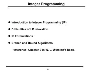
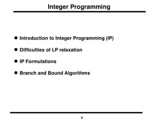
Lecture Outline 1 Introduction 2 Integer Programming 3 Modeling with 0-1 (Binary) Variables 4 Goal Programming 5 Nonlinear Programming
Introduction • Integer programming is the extension of LP that solves problems requiring integer solutions. • Goal programming is the extension of LP that permits more than one objective to be stated. • Nonlinear programming is the case in which objectives or constraints are nonlinear. • All three above mathematical programming models are used when some of the basic assumptions of LP are made more or less restrictive.
Summary: Linear Programming Extensions • Integer Programming • Linear, integer solutions • Goal Programming • Linear, multiple objectives • Nonlinear Programming • Nonlinear objective and/or constraints
Integer Programming • Solution values must be whole numbers in integer programming . • There are three types of integer programs: • pure integer programming; • mixed-integer programming; and • 0–1 integer programming.
Integer Programming • The PureInteger Programming problems are cases in which all variables are required to have integer values. • The Mixed-Integer Programming problems are cases in which some, but not all, of the decision variables are required to have integer values. • The Zero–One Integer Programming problems are special cases in which all the decision variables must have integer solution values of 0 or 1.
9.3 The Branch-and-Bound Method for Solving Pure Integer Programming Problems • In practice, most IPs are solved by some versions of the branch-and-boundprocedure. Branch-and-bound methods implicitly enumerate all possible solutions to an IP. • By solving a single subproblem, many possible solutions may be eliminated from consideration. • Subproblems are generated by branching on an appropriately chosen fractional-valued variable.
Suppose that in a given subproblem (call it old subproblem), assumes a fractional value between the integers i and i+1. Then the two newly generated subproblems are New Subproblem 1 Old subproblem + Constraint New Subproblem 2 Old subproblem + Constraint • Key aspects of the branch-and-bound method for solving pure IPs • If it is unnecessary to branch on a subproblem, we say that it is fathomed.
These three situations (for a max problem) result in a subproblem being fathomed • The subproblem is infeasible, thus it cannot yield the optimal solution to the IP. • The subproblem yield an optimal solution in which all variables have integer values. If this optimal solution has a better z-value than any previously obtained solution that is feasible in the IP, than it becomes a candidate solution, and its z-value becomes the current lower bound (LB) on the optimal z-value for the IP. • The optimal z-value for the subproblem does not exceed (in a max problem) the current LB, so it may be eliminated from consideration. • A subproblem may be eliminated from consideration in these situations • The subproblem is infeasible. • The LB is at least as large as the z-value for the subproblem
Two general approaches are used to determine which subproblem should be solved next. • The most widely used is LIFO. • LIFO leads us down one side of the branch-and-bound tree and quickly find a candidate solution and then we backtrack our way up to the top of the other side • The LIFO approach is often called backtracking. • The second commonly used approach is jumptracking. • When branching on a node, the jumptracking method solves all the problems created by branching.
When solving IP problems using Solver you can adjust a Solver tolerance setting. • The setting is found under the Options. • For example a tolerance value of .20 causes the Solver to stop when a feasible solution is found that has an objective function value within 20% of the optimal solution.
Harrison Electric Company • The Company produces two products popular with home renovators: old-fashioned chandeliers and ceiling fans. • Both the chandeliers and fans require a two-step production process involving wiring and assembly. • It takes about 2 hours to wire each chandelier and 3 hours to wire a ceiling fan. Final assembly of the chandeliers and fans requires 6 and 5 hours, respectively. • The production capability is such that only 12 hours of wiring time and 30 hours of assembly time are available.
Harrison Electric Company If each chandelier produced nets the firm $7 and each fan $6, Harrison’s production mix decision can be formulated using LP as follows: maximize profit = $7X1 + $6X2 subject to: 2X1 + 3X2≤ 12 (wiring hours) 6X1 + 5X2≤ 30 (assembly hours) X1, X2≥ 0 (nonnegative) X1 = number of chandeliers produced X2 = number of ceiling fans produced
Harrison Electric Company With only two variables and two constraints, the graphical LP approach to generate the optimal solution is given below: 6X1 + 5X2≤ 30 + = Possible Integer Solution Optimal LP Solution (X1 = 33/4, X2= 11/2, Profit = $35.25 2X1 + 3X2≤ 12
Integer Solution to Harrison Electric Co. Optimal solution Solution if rounding off
Integer Programming • Rounding off is one way to reach integer solution values, but it often does not yield the best solution. • An important concept to understand is that an integer programming solution can never be better than the solution to the same LP problem. • The integer problem is usually worse in terms of higher cost or lower profit.
Branch and Bound Method • Branch and Bound breaks the feasible solution region into sub-problems until an optimal solution is found. • There are Six Steps in Solving Integer Programming Maximization Problems by Branch and Bound. • The steps are given over the next several slides.
Branch and Bound Method: The Six Steps • Solve the original problem using LP. • If the answer satisfies the integer constraints, it is done. • If not, this value provides an initial upper bound. • Find any feasible solution that meets the integer constraints for use as a lower bound. • Usually, rounding down each variable will accomplish this.
Branch and Bound Method Steps: • Branch on one variable from Step 1 that does not have an integer value. • Split the problem into two sub-problems based on integer values that are immediately above and below the non-integer value. • For example, if X2 = 3.75 was in the final LP solution, introduce the constraint X2 ≥ 4 in the first sub-problem and X2 ≤ 3 in the second sub-problem. • Create nodes at the top of these new branches by solving the new problems.
Branch and Bound Method Steps: 5. • If a branch yields a solution to the LP problem that is not feasible, terminate the branch. • If a branch yields a solution to the LP problem that is feasible, but not an integer solution, go to step 6.
Branch and Bound Method Steps: 5. (continued) • If the branch yields a feasible integer solution, examine the value of the objective function. If this value equals the upper bound, an optimal solution has been reached. If it is not equal to the upper bound, but exceeds the lower bound, set it as the new lower bound and go to step 6. Finally, if it is less than the lower bound, terminate this branch.
Branch and Bound Method Steps: • Examine both branches again and set the upper bound equal to the maximum value of the objective function at all final nodes. • If the upper bound equals the lower bound, stop. • If not, go back to step 3. Minimization problems involve reversing the roles of the upper and lower bounds.
Harrison Electric Co: Figure 11.1 shows graphically that the optimal, non-integer solution is X1 = 3.75 chandeliers X2 = 1.5 ceiling fans profit = $35.25 • Since X1 and X2 are not integers, this solution is not valid. • The profit value of $35.25 will serve as an initial upper bound. • Note that rounding down gives X1 = 3, X2 = 1, profit = $27, which is feasible and can be used as a lower bound.
Subproblem A maximize profit = $7X1 + $6X2 Subject to: 2X1 + 3X2≤ 12 6X1 + 5X2≤ 30 X1≥ 4 Subproblem B maximize profit = $7X1 + $6X2 Subject to: 2X1 + 3X2≤ 12 6X1 + 5X2≤ 30 X1≤ 3 Integer Solution: Creating Sub-problems • The problem is now divided into two sub-problems: A and B. • Consider branching on either variable that does not have an integer solution; pick X1 this time.
Optimal Solution for Sub-problems Optimal solutions are: Sub-problem A: X1 = 4; X2 = 1.2, profit=$35.20 Sub-problem B:X1=3, X2=2, profit=$33.00 (see figure on next slide) • Stop searching on the Subproblem B branch because it has an all-integer feasible solution. • The $33 profit becomes the lower bound. • Subproblem A’s branch is searched further since it has a non-integer solution. • The second upper bound becomes $35.20, replacing $35.25 from the first node.
Subproblem C maximize profit = $7X1 + $6X2 Subject to: 2X1 + 3X2≤ 12 6X1 + 5X2≤ 30 X1≥ 4 X2 ≥ 2 Subproblem D maximize profit = $7X1 + $6X2 Subject to: 2X1 + 3X2≤ 12 6X1 + 5X2≤ 30 X1≥ 4 X2≤ 1 Sub-problems C and D Subproblem A’s branching yields Subproblems C and D.
Sub-problems C and D (continued) • Subproblem C has no feasible solution at all because the first two constraints are violated if the X1 ≥ 4 and X2 ≥ 2 constraints are observed. • Terminate this branch and do not consider its solution. • Subproblem D’s optimal solution is • X1 = 4 , X2 = 1, profit = $35.16. • This non-integer solution yields a new upper bound of $35.16, replacing the original $35.20. • Subproblems C and D, as well as the final branches for the problem, are shown in the figure on the next slide.
Subproblem E maximize profit = $7X1 + $6X2 Subject to: 2X1 + 3X2≤ 12 6X1 + 5X2≤ 30 X1≥ 4 X1≤ 4 X2≤ 1 Optimal solution for E: X1 = 4, X2 = 1, profit = $34 Subproblems E and F • Finally, create subproblems E and F and solve for X1 and X2 with the added constraints X1 ≤ 4 and X1 ≥ 5. The subproblems and their solutions are:
Subproblem F maximize profit = $7X1 + $6X2 Subject to: 2X1 + 3X2≤ 12 6X1 + 5X2≤ 30 X1≥ 4 X1≥ 5 X2≤ 1 Optimal solution for F: X1 = 5, X2 = 0, profit = $35 Subproblems E and F (continued)
Goal Programming • Firms usually have more than one goal. For example, • maximizing total profit, • maximizing market share, • maintaining full employment, • providing quality ecological management, • minimizing noise level in the neighborhood, and • meeting numerous other non-economic goals. • It is not possible for LP to have multiple goals unless they are all measured in the same units (such as dollars), • a highly unusual situation. • An important technique that has been developed to supplement LP is called goal programming.
Goal Programming (continued) • Goal programming “satisfices,” • as opposed to LP, which tries to “optimize.” • Satisfice means coming as close as possible to reaching goals. • The objective function is the main difference between goal programming and LP. • In goal programming, the purpose is to minimize deviational variables, • which are the only terms in the objective function.
Example of Goal Programming Harrison Electric Revisited Goals Harrison’s management wants to achieve, each equal in priority: • Goal 1: to produce as much profit above $30 as possible during the production period. • Goal 2: to fully utilize the available wiring department hours. • Goal 3: to avoid overtime in the assembly department. • Goal 4: to meet a contract requirement to produce at least seven ceiling fans.
Example of Goal Programming Harrison Electric Revisited Need a clear definition of deviational variables, such as : d1–= underachievement of the profit target d1+= overachievement of the profit target d2–=idle time in the wiring dept. (underused) d2+= overtime in the wiring dept. (overused) d3–=idle time in the assembly dept. (underused) d3+= overtime in the wiring dept. (overused) d4–= underachievement of the ceiling fan goal d4+= overachievement of the ceiling fan goal
Ranking Goals with Priority Levels A key idea in goal programming is that one goal is more important than another. Priorities are assigned to each deviational variable. Priority 1 is infinitely more important than Priority 2, which is infinitely more important than the next goal, and so on.
Goal Programming Versus Linear Programming • Multiple goals (instead of one goal) • Deviational variables minimized (instead of maximizing profit or minimizing cost of LP) • “Satisficing” (instead of optimizing) • Deviational variables are real (and replace slack variables)
9.2 Formulating Integer Programming Problems • Practical solutions can be formulated as IPs. • The basics of formulating an IP model
Example 1: Capital Budgeting IP • Stockco is considering four investments • Each investment • Yields a determined NPV • Requires a certain cash flow at the present time • Currently Stockco has $14,000 available for investment. • Formulate an IP whose solution will tell Stockco how to maximize the NPV obtained from the four investments.
Example 1: Solution • Begin by defining a variable for each decision that Stockco must make. • The NPV obtained by Stockco isTotal NPV obtained by Stocko = 16x1 + 22x2 + 12x3 + 8x4 • Stockco’s objective function ismax z = 16x1 + 22x2 + 12x3 +8x4 • Stockco faces the constraint that at most $14,000 can be invested. • Stockco’s 0-1 IP is max z = 16x1 + 22x2 + 12x3 +8x4 s.t. 5x1 + 7x2 + 4x3 +3x4 ≤ 14 xj = 0 or 1 (j = 1,2,3,4)
Set Covering as an IP • In a set-covering problem, each member of a given set must be “covered” by an acceptable member of some set. • The objective of a set-covering problem is to minimize the number of elements in set 2 that are required to cover all the elements in set 1.
Piece-wise linear functions as IP • 0-1 variables can be used to model optimization problems involving piecewise linear functions. • A piecewise linear function consists of several straight line segments. • The graph of the piecewise linear function is made of straight-line segments. • The points where the slope of the piecewise linear function changes are called the break points of the function. • A piecewise linear function is not a linear function so linear programming cannot be used to solve the optimization problem.
Piece-wise linear functions as IP • By using 0-1 variables, however, a piecewise linear function can be represented in a linear form. Suppose the piecewise linear function f (x) has break points .
Piece-wise linear functions as IP • Suppose the piecewise linear function f (x) has break points . • Step 1 Wherever f (x) occurs in the optimization problem, replace f (x) by . • Step 2 Add the following constraints to the problem:
Piece-wise linear functions as IP • If a piecewise linear function f(x) involved in a formulation has the property that the slope of the f(x) becomes less favorable to the decision maker as x increases, then the tedious IP formulation is unnecessary. • LINDO can be used to solve pure and mixed IPs. • In addition to the optimal solution, the LINDO output also includes shadow prices and reduced costs. • LINGO and the Excel Solver can also be used to solve IPs.
9.4 The Branch-and-Bound Method for Solving Mixed Integer Programming Problems • In mixed IP, some variables are required to be integers and others are allowed to be either integer or non-integers. • To solve a mixed IP by the branch-and-bound method, modify the method by branching only on variables that are required to be integers. • For a solution to a subproblem to be a candidate solution, it need only assign integer values to those variables that are required to be integers
9.5 Solving Knapsack Problems by the Branch-and-Bound Method • A knapsack problem is an IP with a single constraint. • A knapsack problem in which each variable must be equal to 0 or 1 may be written as • When knapsack problems are solved by the branch-and-bound method, two aspects of the method greatly simplify. • Due to each variable equaling 0 or 1, branching on xi will yield in xi =0 and an xi =1 branch. • The LP relaxation may be solved by inspection. max z = c1x1 + c2x2 + ∙∙∙ + cnxn s.t. a1x1 + a2x2 + ∙∙∙ + anxn ≤ b x1 = 0 or 1 (i = 1, 2, …, n)