Download
1 / 39
390 likes | 407 Views
Explore how satellite data can provide insight into emissions of reactive organic gases in North America, focusing on isoprene emissions and HCHO measurements. Learn about the challenges and techniques involved in mapping VOC emissions from space.

E N D
What can satellites tell us about emissions of reactive organic gases from North America? Dylan Millet with D.J. Jacob and K.F. Boersma Atmospheric Chemistry Modeling Group, Harvard University T.P. Kurosu and K. Chance Harvard-Smithsonian Center for Astrophysics C. Heald (UC Berkeley), A. Guenther (NCAR), A. Fried (NCAR), B. Heikes (URI), D. Blake (UCI), and H. Singh (NASA-Ames) Daly Fellows Talk Department of Earth and Planetary Sciences Harvard University November 7, 2006
NO2 OH h HO2 RO2 O3 NO Volatile organic compounds (VOCs) smog human, ecosystem, crop health greenhouse gas cleansing agent sink for pollutants & greenhouse gases OH organic aerosol health visibility climate VOCs Affect Atmospheric Composition and Climate t ~ minutes to years
Sources of Reactive VOCs to the Atmosphere Isoprene Most important biogenic non-methane VOC Global emissions ~ methane (but > 104times more reactive) ~ 6x anthropogenic VOC emissions
Global Distribution of Isoprene Emissions E = f (T, h) MEGAN biogenic emission model (Guenther et al., 2006)
Global Distribution of Isoprene Emissions MEGAN biogenic emission model (Guenther et al., 2006)
Bottom-Up Biogenic VOC Emission Estimates Leaf & plant enclosure measurements Pro accurate quantify response to isolated drivers (T, h, CO2, soil moisture) Con labor intensive scaling up Eddy flux measurements Pro integral of emissions from entire ecosystem minutes-years Con scaling up measurement difficulty with complex terrain and at night Can we derive top-down constraints from satellites to test these bottom-up inventories?
Measuring Tropospheric Composition from Space Global, continuous information for a range of issues: Constraints on Sources Air Quality Monitoring, Forecasting Long Range Pollution Transport Radiative Forcing ozone, aerosols Air pollution, greenhouse gases NO2 PM2.5 CO Challenges: water vapor, ozone layer, aerosols, clouds, surface solar backscatter thermal emission solar occultation space lidar 4 techniques available:
Solar Backscatter Measurements (UV to near-IR) z absorption λ [X] Retrieved column depends on vertical profile need chemical transport and radiative transfer models Scattering by Earth’s surface and the atmosphere Pro Con daytime only no vertical information interference from stratosphere small field of view sensitive to lower troposphere
Thermal Emission Measurements (IR, mwave) Nadir View elIl(T1) Limb View T1 Absorber Il(To) To Earth Surface Pro Con versatility small field of view vertical profiling water vapor interference insensitive to lower troposphere
Occultation Measurements (UV to near-IR) Pro Con sparse coverage upper troposphere only low horizontal resolution good S/N vertical profiling
LIDAR Measurements (UV to near-IR) laser pulse Pro Con day or night high vertical resolution aerosols only limited coverage
Mapping VOC Emissions from Space SBUV satellite instrument OH, h ki, Yi VOCs HCHO Sensitivity
Measuring HCHO from Space SBUV instruments in low Earth orbit GOME SCIAMACHY OMI 1995-2001 40 x 320 km footprint global coverage: 3 days 2002-present 30 x 60 kmfootprint global coverage: 6 days 2004-present 13 x 24 kmfootprint global coverage: 1 day
HCHO Distribution over North America Modeled isoprene emissions (bottom-up)
Relating HCHO Columns to Isoprene Emission ΩHCHO Isoprene a-pinene detection limit propane 100 km Distance downwind VOC source HCHO vertical columns measured by OMI (K. Chance, T.P. Kurosu et al.) OH, h ki, Yi OH, h kHCHO HCHO VOCs Local ΩHCHO-Ei Relationship Palmer et al., JGR (2003,2006).
Mapping Isoprene Emissions from Space Testing the Approach: OH, h ki, Yi OH, h kHCHO HCHO VOCs ΩHCHO Isoprene a-pinene detection limit propane 100 km Distance downwind VOC source 1) What is the error in HCHO columns measured from space? 2) What drives column HCHO variability over North America? 3) What are the implications for retrieving isoprene emissions from space? Address using aircraft measurements Local ΩHCHO-Ei Relationship Palmer et al., JGR (2003,2006).
Testing the Approach:Error Characterization Main Sources of Error Use INTEX-A aircraft data & GEOS-Chem model to test errors in HCHO measured from space Fitting uncertainty ~ 4 x 10¹⁵ molecules cm-2 HCHO GOME/OMI sensitivity Ratio between HCHO along light path and the vertical column amount HCHO vertical profile scattering by air molecules, aerosols, clouds surface albedo INTEX-A aircraft experiment over North America summer 2004 GEOS-Chem global 3D model of atmospheric chemistry source of external information in HCHO retrieval
Testing the Approach:Error Characterization Mean bias Precision • Atmospheric Scattering • clouds, aerosols • HCHO vertical profile • Surface albedo Clouds: primary source of error 1σ error in HCHO satellite measurements: 25–31% Recommended cloud cutoff: 50% Sensitivity Shape Factor bEXT (Mm-1) Millet et al., JGR (2006).
Testing the Approach:Relating isoprene emission to HCHO column INTEX-A ΩHCHO = SEisoprene+ B Measured HCHO production rate vs. column amount What drives variability in column HCHO? Isoprene dominant source when ΩHCHO is high Other VOCs give rise to a relatively stable background ΩHCHO Not to variability detectable from space Millet et al., JGR (2006). ΩHCHO variability over N. America driven by isoprene
Testing the Approach:Relating isoprene emission to HCHO column INTEX-A Observed GEOS-Chem M = 3.5 M = 3.6 ΩHCHO = SEisoprene+ B ΩHCHO (1016 molec cm-2) ΩISOPRENE (1016 molec cm-2) Test HCHO yield from isoprene From aircraft profiles during INTEX-A: HCHO yield from isoprene = 1.6 ± 0.5 Consistent with current chemical mechanisms Millet et al., JGR (2006).
What Did We Learn from GOME? Year-To-Year Variability of GOME HCHO Over Southeast US • Good accord for seasonal variation, regional distribution of emissions; • Differences in hot spot locations Palmer et al. [2006]
Year-To-Year Variability of GOME HCHO Over Southeast US Amplitude and phase are highly reproducible GOME HCHO Column [1016 molec cm-2] Southeast US average 32-38N; 100-85W Palmer et al. [2006]
What Drives Temporal Variance of Isoprene Emission Over Southeast US? Monthly mean GOME HCHO vs. surface air temperature; MEGAN parameterization shown as fitted curve Temperature accounts for ~80% of the variance Palmer et al. [2006]
Using OMI HCHO to Define Spatial Distribution of Eisoprene HCHO columns measured with the OMI satellite instrument (summer 2006) Isoprene emissions from the MEGAN biogenic emission inventory (summer 2006) ? Comparison between emission inventory and HCHO columns from GOME & OMI indicates mismatch in hotspot locations Implications for OH, O3, SOA production
Model of Emissions of Gases and Aerosols from Nature Environmental drivers (T, h, LAI, leaf age, …) Vegetation-specific baseline emission factors Land cover database MEGAN Isoprene emissions Guenther et al., Atmos. Chem. Phys., 6, 3181–3210, 2006. [1013 atomsC cm-2 s-1]
OMI vs. GEOS-Chem with MEGAN Emissions Similarity in broad pattern (r2 = 0.86) … but important differences [1015 molecules cm-2]
Relating HCHO Columns to Isoprene Emissions [1015 molecules cm-2] [1013 atomsC cm-2 s-1] ΩHCHO = SEisoprene+ B Domain-wide ΩHCHO-Eisoprene relationship Local ΩHCHO-Eisoprene relationship [1013 atomsC cm-2 s-1]
Testing Current Bottom-Up Inventories Drive MEGAN with 2 land cover databases Guenther [2006] (MODIS) Community Land Model (AVHRR) MEGAN Isoprene Emissions w/ Guenther vegetation MEGAN Isoprene Emissions w/ Community Land Model vegetation …evaluate spatial distribution of emissions with top-down constraints from OMI
Spatial Patterns in Isoprene Emissions MEGAN w/ Guenther vegetation Domain-wide ΩHCHO-Eisoprene relationship Local ΩHCHO-Eisoprene relationship OMI - MEGAN OMI - MEGAN
Spatial Patterns in Isoprene Emissions MEGAN w/ Community Land Model vegetation Domain-wide ΩHCHO-Eisoprene relationship Local ΩHCHO-Eisoprene relationship OMI - MEGAN OMI - MEGAN
Spatial Patterns in Isoprene Emissions OMI – MEGAN Isoprene Emissions June-August, 2006 Large sensitivity to surface database used MEGAN w/ Guenther Land Cover Guenther & CLM vegetation MEGAN higher than OMI over ‘hotspots’ such as the Ozarks MEGAN w/ CLM Land Cover CLM vegetation MEGAN lower than OMI over deep South & Atlantic coast
Why Are Emissions Overestimated in Ozarks & Other Hotspots? Bottom-up emissions are too high in Ozarks, Virginia OMI – MEGAN Isoprene Emissions June-August, 2006 MEGAN w/ Guenther Land Cover Large emissions driven by oak tree cover, high temperatures OMI comparison suggests broadleaf tree emissions are overestimated Guenther Broadleaf Trees MEGAN w/ CLM Land Cover
Why Are Emissions Underestimated in Deep South & Atlantic Coast? CLM-driven bottom-up emissions are too low in deep South, Atlantic coast OMI – MEGAN Isoprene Emissions June-August, 2006 MEGAN w/ Guenther Land Cover Discrepancies in broadleaf tree and shrub cover lead to large differences in calculated isoprene emissions! CLM – Guenther Broadleaf Tree Cover MEGAN w/ CLM Land Cover CLM – Guenther Shrub Cover
Conclusions OMI HCHO columns are broadly consistent with state-of-the-art bottom-up emission inventories (R2 = 0.86) … but with important spatial differences Bottom-up isoprene emission estimates are too high in the Ozarks and other ‘hotspots’ Overestimate of broadleaf tree emissions CLM-driven bottom-up isoprene emission estimates are too low over the deep South and along the Atlantic coast Underestimate of broadleaf tree and shrub cover
Next Steps What are the implications of these new OMI-derived constraints for our understanding of ozone, OH and organic aerosol production? How can we apply these satellite data to learn about VOC emissions in other parts of the world?
Acknowledgements EPS @ Harvard University NOAA Postdoctoral Program in Climate and Global Change NASA/ACMAP OMI science team B. Yantosca, P. Palmer (now at Leeds), M. Fu, and other coworkers at Harvard The INTEX-A science team