Download
1 / 41
410 likes | 589 Views
Lecture 5 Maximum Likelihood and model selection. Joe Felsenstein. Maximum Likelihood : The explanation that makes the observed outcome the most likely. L = Pr( D | H ). Probability of the data, given an hypothesis

E N D
Lecture 5 Maximum Likelihood and model selection Joe Felsenstein
Maximum Likelihood: The explanation that makes the observed outcome the most likely L = Pr(D|H) Probability of the data, given an hypothesis The hypothesis is a tree topology, its branch-lengths and a model under which the data evolved First use in phylogenetics: Cavalli-Sforza and Edwards (1967) for gene frequency data; Felsenstein (1981) for DNA sequences
example Suppose you are flipping coins and counting the number of times “heads” appear – This is your data. You throw the coin twice and observe “heads” both times. You might have two hypotheses to explain these data. “heads” “tails” “heads” “tails”
H1 is the hypothesis that the coin is normal: “heads” on one side, “tails” on the other and each has the same probability, p = 0.5, of appearing. • H2 is the hypothesis that the coin is rigged with an 80% chance of getting a head , p = 0.8. • What is the likelihood of H1? • What is the likelihood of H2?
The probability of observing “heads” in each of two flips under H1 is: L(H1|data) = 0.5 0.5 = 0·25 • The probability of observing “heads” in each of two flips under H2 is: L(H2|data) = 0.8 0.8 = 0.64
Since the probability of observing the data under H2 is greater than under H1, you might argue that the “rigged” coin hypothesis is the more likely. However, if you flipped the same coin 20 times and got “heads” 8 times, would H2 still be the better explanation of the data?
Note that you could flip “heads” and “tails” in different orders • E.g. HTHHTHTTHTTTTHHTTHTT • Or HHHHHHHHTTTTTTTTTTTT There are actually 20 choose 8 ways to do this
The likelihood for H1 of observing 8 “heads” and 12 “tails” (where each has an equal chance of appearing) under H1 is: L(H1 data) = 20C8 (0.5)8(0.5)12 20 19 18….21 = (0.5)8(0.5)12 (8 7 6….21)(121110….21)
Numbers can be very low, so normally take natural logs lnL(H1)= 2.119 The likelihood for H2 of observing 8 “heads” and 12 “tails” (where “heads has a probability of 0.8 of appearing) under H2 is: L(H2 data) = 20C8 (0.8)8(0.2)12 lnL(H2)= 9.355 Maximum likelihood is less likely to be misleading with more data
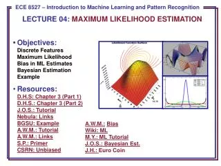
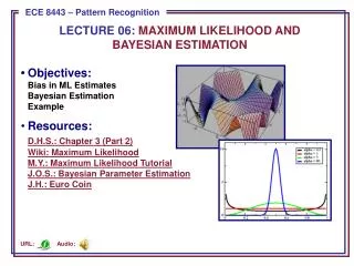
The maximum likelihood estimate (MLE) Plotting likelihood (or –lnL) values for different parameter values (e.g. equilibrium base frequency for Adenine, πA) gives the likelihood surface. The best score on this surface (the lowest point) identifies the maximum likelihood estimate(MLE), and indicates the hypothesis best supported by the data. Here the MLE for πA ≈ 0.35 πA
In phylogenetics, the hypothesis is a tree topology, its branch-lengths and a model under which the data evolved Sheep Goat Branch-lengths as expected numbers of substitutions per site 0.10 0.14 0.32 0.05 0.08 Cow Bison Parsimony seeks to minimise the number of substitutions Likelihood seeks to estimate the actual number of substitutions
Parsimony assumes that having knowledge about how some sites are evolving tells us nothing about other sites. Likelihood assumes that sites evolve independently, but by common mechanisms Purines Oak ATGACCGCTGCCAG Ash ACGCTCGCCATCAG Maple ATGCTCGCTACCGG A G Transitions at six sites, only one transversion is observed Hence, an ML model should allow for different transition and transversion substitution rates C T Pyrimidines Transitions Transversions
The model is reversible, ie. p(AG) = p(AG), so the root can be placed at any node Pattern probability = p(G G) p(G G) p(G A) p(A A) p(A A) A A Under the simple Jukes-Cantor model, all base frequencies=0.25, all substitutions equally probable. b is branch-length (subs/site) G A Pij (i=j) = 0.25+0.75eb G G Root Pij (i≠j) = 0.25-0.25eb b is branch-length (subs/site)
Pij (i=j) = 0.25+0.75eb A A Pij (i≠j) = 0.25-0.25eb 0.5 0.5 G b is branch-length (subs/site) A 0.5 0.5 0.5 G G Root Where b=0.5, Pij (I=j) = 0.7049, Pij(i≠j) = 0.0984 Site pattern probability = p(G G) p(G G) p(G A) p(A A) p(A A) =0.7049 0.7049 0.0984 0.7049 0.7049 = 0.0243
A A A A A A A A A A A A A GC T A G A A A A C C G G G G G G G G G G G G A A A A A A A A A A C T A GC The site likelihood is the sum of the probabilities for the 16 possible site patterns = 0.0333 C CT T T G G G G G G G G G G A A A A A A A A A A T A GCT TG G G G G G G G G G G G G G Hence, the site lnL = 3.402
The likelihood of a tree is the product of the site likelihoods. Taken as natural logs, the site likelihoods can be summed to give the log likelihood: the tree with the highest likelihood (lowest –lnL) is the ML tree. Tree 1 Tree 2 Site –lnL(1) –lnL(2) 2.457 2.891 2 1.568 1.943 . .. .. . .. .. Tree 2 is the ML tree by 8.801 –lnL units 1206 2.541 1.943 2052.456 2043.655
Long-branch attraction Simulation tree Parsimony reconstruction 1 1 2 4 3 2 4 3 Sequence at root: AGACTGATCGAATCGATTAG Sequence at 1: ATACGGACAGAACGGTTAAG Sequence at 2: AGACTGATCGATTCGATTAG Sequence at 3: AGAATGATCGATTCGATTAG Sequence at 4: CGAATGATCGAATGGACTTG Parallel change True synapomorphy Back mutation
Under the correct model, Maximum likelihood will account for parallel changes and back mutations Maximum likelihood tree Maximum parsimony tree Long-branch attraction Goremykin (Molec. Biol. Evol., 2005) chloroplast genome sequences
Major programs supporting maximum likelihood analysis • PHYLIP (http://evolution.gs.washington.edu/phylip/software.html) • PAUP* (http://paup.csit.fsu.edu) • PHYML (http://atgc.lirmm.fr/phyml/) • PAML (http://abacus.gene.ucl.ac.uk/software/paml.html) • TREE-PUZZLE (http://www.tree-puzzle.de) • DAMBE (http://aix1.uottawa.ca/~xxia/software/software.htm)
General time-reversible (GTR+I+ ) likelihood parameters Branch-lengths: (2n-3 free parameters on unrooted trees) Substitution rates: A-C, A-G, A-T, C-G, C-T, G-T (5 free parameters) Base frequencies: πA πG πC πT (3 free parameters) Proportion of invariant sites: I (1 free parameter) Shape of the distribution: (1 free parameter)
Substitution model categories GTR: 6 substitution types, unequal base frequencies 3 substitution types (transversion, 2 transitions) Equal base frequencies TrN SYM 2 substitution types transversion, transition) 3 substitution types (transition, 2 transversions) HKY85 / F84 TrN Single substitution type 2 substitution types transversion, transition) Equal base frequencies F81 K2P Note: there are also models for codon and amino acid data Equal base frequencies Single substitution type JC
Which is the most appropriate model? Too few parameters can lead to inaccuracy, convergence upon the wrong tree (inconsistency) Too many parameters can reduce statistical power, the ability to reject an hypothesis likelihood ratio test (LRT) The test statistic () is 2(lnLmodel_1minus lnLmodel_2 ) is compared to a 2 distribution critical value (where the degrees of freedom is the difference in the number of free parameters being estimated between the two models.
= 2(lnLmodel_1minus lnLmodel_2 ). HO: models 1 and 2 explain the data equally well AcceptHOcritical value RejectHO
The Akaike Information Criterion (AIC) AIC for each model = 2lnL + (2 the number of free parameters) Choose the model with the lower AIC • Can be compared between non-nested models • Does not assume a 2 distribution • May tend to over-parameterization more than LRT
How well does the model reflect the substitution process? Parametric bootstrap: compares the observed sequence data with data predicted from the model (observed vs. expected site pattern frequencies) 1 AGCA 2 AGAT 3 TGAT 4 TGCT
The test statistic = likelihood ratio between the multinomial likelihood T(X) and the standard substitution model likelihood n T(X) = N ln(N) N ln(N) i i is the ith unique site pattern, Ni is the number of times that pattern appears, n is the number of unique site patterns and N is the total number of sites.
1. Calculate the test statistic O for the observed data 2. Simulate many pesudoreplicate datasets using the ML topology, branch lengths and model parameters 3. Calculate the test statistic i for each of the pseudoreplicates 4. If O is greater than (e.g.) 95% of the ranked values of i then the null hypothesis is rejected O= 126.7 p = 0.317 frequency 125 105 110 115 120 130 135 140 145
Maximum likelihood analysis is computationally expensive Time (t) for one ML(GTR+I+ ) heuristic search on a X-taxa, 3425 nt in length (using a Pentium 4 processor) Taxa Parameters estimated fixed X = 5; t = 46s t = 0.3s X = 6; t = 4m 37s t = 1.3s X = 7; t = 15m 58s t = 2.5s X = 8; t = 39m 16s t = 5.5s So for ML on large datasets it is not feasible to use non-parametric bootstrapping (reconstruct the tree from many resamplings from the observed data (draw and replace n nucleotide sites, where n=sequence length)
Accounting for stochastic (sampling) error Flip 2 coins 100 times, does coin A give more tails than coin B Can the difference in likelihood between two hypotheses be explained by sampling error? Compare with a null distribution Proportion of tails
Choosing just a finite number of nucleotide sites (e.g. 500) also has the problem of sampling error Here = lnLT1minus lnLT2 Null distribution for the likelihood ratio statistic AcceptHOcritical valueRejectHO
Maximum likelihood Hypothesis testing If comparing a small number of alternative trees, ML hypothesis tests allow full parameter optimisation Kishino-Hasegawa (KH) test Winning sites tests Shimodaira-Hasegawa (SH) test Approximately unbiased (AU) test Swofford, Olsen, Waddell, Hillis (SOWH) test Parametric bootstrap test
1 3 1 3 T1 T2 Kishino-Hasegawa test 2 4 2 4 HO: T1 and T2 explain the data equally well; ie. =0 1. Calculate the likelihood ratio statistic between T1 and T2 2. Bootstrap the data (or site likelihoods) to generate pseudoreplicates 3. Optimise ML on each pseudoreplicate for T1 and T2 4. Calculate i for each pseudoreplicate 5. Centre the distribution by subtracting the mean of i from each value of i 6. If lies outside of 2.5% - 97.5% of the ranked distribution of I, then HOis rejected
Shimodaira-Hasegawa test Corrects for comparing multiple topologies HO: That all topologies are equally good explanations of the data HA: That some topologies do not explain the data as well as others Approximately unbiased test Generates pseudoreplicates that differ in length from the original dataset, in order to explore site-pattern space. This allows more accurate correction for comparing multiple topologies HO and HAas above
1 3 1 3 T1 TML SOWH test 2 4 2 4 HO: That T1 is the true tree HA: That some other tree is the true tree 1. Optimise T1 and TML on the original data and calculate the likelihood ratio 2. Simulate many datasets using T1 (topology, branch-lengths, substitution parameters) 3.For each dataset (i) optimise the likelihood for T1 to give L1i and find TML to give LMLi 4. Calculate i for each TML to give LMLi pair. 5. If is greater than 95% of the ranked values of i, reject HO.
Which hypothesis test to use? If just pairwise hypothesis testing and neither is a priori known to be the ML tree, then the KH test If comparing many topologies simultaneously and the curvature of site-pattern space can be defined, then AU test, otherwise, SH test, which is very conservative and the power to reject HO is dependent on the number of topologies tested) SOWH tests the full phylogenetic model (topology, branch-lengths, substitution parameters), so can be difficult to interpret when the object is specifically to compare topologies. If the model is misspecified it will not be conservative enough.
A Maximum likelihood analysis: What are the phylogenetic affinities of turtles Turtles and many early reptilian groups Mammals Squamates: e.g. lizards/snakes Some marine reptiles, derived from diapsids
Squamata Turtle placement hypotheses Amphibia (outgroup) H2: Diapsida H3: Archosauria H1: Anapsida Aves Mammalia Crocodilia
Complete mitochondrial genome RNA sequences: 3,110 nucleotides Modeltest (Posada and Crandal, Bioinformatics, 1998) • Hierarchical Likelihood Ratio Tests (hLRTs) • Equal base frequencies • Null model = JC -lnL0 = 28513.7910 • Alternative model = F81 -lnL1 = 28409.5176 • = 2(lnL1-lnL0) = 208.5469 df = 3 P-value = <0.000001 Optimized Model LRT → TrN+I+; on AIC →GTR+I+ Base frequencies = (0.3546 0.2105 0.1780 0.2569) Rate matrix = (1.0000 5.3176 1.0000 1.0000 8.7021 1.0000) Rates=gamma Pinvar=0.2284 Shape=0.9845
ML (TrN+I+) heuristic search Dog 3 toed Sloth Mammalia Kangaroo Opossum Platypus Echidna Skink Iguana Green Turtle Painted Turtle Diapsidia Alligator Archosauria Caiman Cassowary Penguin Caecilian Amphibia Salamander 0.05 substitutions/site
Tree 1 Tree 3 Amphibia Amphibia Turtles Mammalia Mammalia Squamates 98 Squamates Turtles 88 Non-parametric bootstrap support Birds Birds Crocodilia Crocodilia Tree 2 Amphibia Tree1 Tree2 Tree3 -lnL +36.1 +11.7 <best> KH 0.002 0.044 -- SH 0.003 0.153 -- AU 0.001 0.054 -- SOWH <0.001 <0.001 -- Mammalia Turtles Squamates Birds Crocodilia
Turtles are not a remnant of early anapsid reptiles, instead they group within Diapsida • The anapsid condition must be a reversal in turtles, as has occurred convergently with other armoured diapsid groups • Within Diapsida, turtles are likely sister to Archosauria (inc. birds and crocodiles) - this explains the missing 80Ma fossil record of turtles (prior to 230 Ma) Ankylosaurus