Download
1 / 42
430 likes | 705 Views
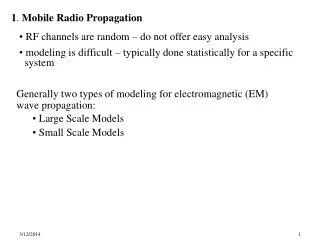
1 . Mobile Radio Propagation RF channels are random – do not offer easy analysis modeling is difficult – typically done statistically for a specific system. Generally two types of modeling for electromagnetic (EM) wave propagation: Large Scale Models Small Scale Models.

E N D
1. Mobile Radio Propagation • RF channels are random – do not offer easy analysis • modeling is difficult – typically done statistically for a specific • system • Generally two types of modeling for electromagnetic (EM) • wave propagation: • Large Scale Models • Small Scale Models
Large Scale Propagation Models: predict mean signal strength • for TX-RX pair with arbitrary separation • useful for estimating coverage area of a transmitter • characterizes signal strength over large distances (102-103 m) • predicts local average signal strength generally decreases with • distance • signal power commonly computed by averaging measurements over • a measurement track of 5 - 40 • e.g. at 2.4 GHz, =12.5cm measurement tracks range from • 0.625m - 5m
Small Scale or Fading Models: characterize rapid fluctuations of • received signal over • short distances (few ) or • short durations (few seconds) • with mobility over short distances • instantaneous signal strength fluctuates • received signal = sum of many components from different directions • phases are random sum of contributions varies widely • received signal may fluctuate 30-40 dB by moving a fraction of
received power dBm -30 -35 -40 -45 -50 -55 -60 -65 Small Scale & Large Scale Fading 1 point = average over 5 = 0.625m 14 15 16 17 18 19 20 21 22 23 24 25 26 d (meters) fc= 2.4GHz 0.125m
Pr(d) = (1.1) 1.1 Free Space Propagation Model: Friis free space equation: • Pr & Pt= power at receive & transmit antenna • Gt & Gr = gain of transmit & receive antenna • = wavelength • d = antenna separation • L = systemlosses not from propagation • - line attenuation, filter antenna • - if L = 1 no system losses • - practically L 1 i • power decays by d 2 decay rate = 20dB/decade
G= (1.2) Antenna Gain: Ae = effective aperture size – related to antenna size PL = = (1.3a) PL (dB) = 10 log 10 (Pt /Pr) = (1.3b) Path Loss (PL): ratio of transmit power to receive power if G is assumed to be unit gain: (1.4) PL (dB) =
open circuit Rant to matched receiver Vant V Pr(d) = (1.5) • 1.2 Receiver input voltage vsreceive power level • model receive antenna as matched resistive load • receiver antenna induces rms voltage into receiver • induced voltage = ½ open circuit voltage at antenna: V = ½ Vant • Vant = receive antenna voltage • Rant = antenna resistance • E = induced electric field • V = induced receiver input voltage • |E |= magnitude of radiating portion of electric field in far-field
1.3 Radio Wave Propagation: diverse mechanisms of EM wave propagation generally attributed to • diffraction • reflection • scattering
E1i plane of incidence E2i dielectric boundary (reflecting surface) i r t • Reflection: EM wave in 1st medium impinges on 2nd medium • part of the wave is refracted & part is reflected • EM plane-wave incident on a perfect conductor • all energy is reflected back into 1st medium • no loss of energy from absorption • EM plane-wave incident on a perfect dielectric(non-conductor) • part of energy is transmitted (refracted) into 2nd medium • part of energy is transmitted (reflected) back into 1st medium • ideally no energy loss from absorption - practically dielectrics • absorbs some energy
PL = (1.6) PL(dB) = 40log d - (10logGt+ 10logGr + 20log ht + 20 log hr) 2 Ray Ground Reflection Model • considers both LOS path & ground reflected path • based on geometric optics • reasonably accurate for predicting large scale signal strength for • distances of several km • useful for • - mobile RF systems which use tall towers (> 50m) • - LOS microcell channels in urban environments path loss for 2-ray model with antenna gains is expressed as:
Diffraction • allows RF signals to propagate to obstructed (shadowed) regions • - over the horizon (around curved surface of earth) • - behind obstructions • Huygen’s Principal • all points on a wavefront can be • point sources for producing 2ndry wavelets • 2ndry wavelets combine to produce new wavefront in the direction • of propagation • diffractionarises from propagation of 2ndry wavefrontinto • shadowed area • field strength of diffracted wave in shadow region = electric field • components of all 2ndry wavelets in the space around the obstacle
Scattering • RF waves impinge on rough surfacereflected energy diffuses in all directions • e.g. lamp posts, leaves in a tree results in random multipath • components • provide additional RF energy at receiver • actual received signal in mobile environment often stronger than • predicted by diffraction & reflection models alone
Coherence BW Fading 100% 90% Signal Level f 2. Mobile Radio Propagation – Small Scale Fading - Multipath • Fading: rapid fluctuations in amplitude over short time & distance • large-scale effects are negligible • caused by interference from 2+ versions of the transmitted signal • arriving at different phase from multiple paths • wide variation in phase & amplitude – depending on distribution • effected by channel bandwidth & channel multipath structure • Bc= coherence bandwidth: related to channel’s multipath structure • - measure of maximum frequency difference between signals with • strongly correlated amplitudes
2.1 Small Scale Multipath Propagation • rapid changes in amplitude over small distance & time intervals • doppler shift on different multipaths random frequency shifts • time dispersion (echoes) caused by multipath • urban areas • no LOS path - mobile antenna height < surrounding structures • even with LOS path multipath exists • received signal at any point consists of many plane waves with • - randomly distributed amplitudes phases, angles • - components combine vectorially at receiver • - causes distorted or faded signal reception
Four Factors of Fading • (i) multipath propagation: objects cause reflection & scattering • multiple versions arrive at different times and spatial orientation • causes signal smearing - intersymbol interference (ISI) (ii) relative speed between Tranmitter - Reciever doppler shift (iii) moving objects induce time varying Doppler shift on multipath components • (iv) bandwidth of transmitted signal • if signal bandwidth > multipath channel bandwidth • - received signal will be distorted • - signal won’t fade over a small area – ignore small scale fading • if signal bandwidth << multipath channel bandwidth • - rapidly changing signal amplitude (fading) • - but signal will not be distorted
hb(t, ) t t3 (t3) t2 (t2) t1 (t1) t0 time amplitude (t0) 0 1 2 3 4 … N-2 N-1 delayedmultipath components • time-varying discrete impulse response model for multipath channel • hb(t, ) = baseband impulse response of multipath channel • time = t varies into the page • time delay bins are quantized to widths =
10 5 0 -5 -10 -15 -20 -25 -30 -35 signal level (dB about rms) 0 50 100 150 200 (ms) • 2.2 Rayleigh Fading Distributions • commonly used to model mobile RF channels • describes statistical time varying nature of received envelope for • (i) flat fading signal • (ii) single multipath component Rayleigh distributed signal vs time
p(r) = (2.1) 0 . 6065 p(r) • CDF – cumulative distribution function of Rayleigh Distribution • probability that received signal’s envelope doesn’t exceed • specified value, R P(R) = Pr(r R) = (2.2) 0 2 3 4 5 Rayleigh distribution PDF - probability distribution function r = received signal envelope voltage = rms value of received voltage before envelope detection 2 = time average power of received signal before envelope detection
(4.55) p(r) = A = peak amplitude of dominant signal 0() = modified Bessel function of the 1st kind & zero order • 2.3 Ricean Fading Distributions • if signal has – LOS path small scale fading envelope is Ricean • random multipath components arriving at different angles are • superimposed on LOS signal • as LOS component fades distribution degenerates to Rayleigh
K = K (dB) = (4.56) p(r) • as signal attenuates A grows small • Ricean distribution degenerates to Rayleigh K = - dB K = 6 dB 0 2 3 4 5 • Ricean Distribution often described in terms of parameter K • K is known as Ricean Factor • K = ratio of deterministic signal power & multipath variance
Definitions of Bandwidth • absolutebandwidth = , range of frequencies over which PSD 0 • null-to-nullbandwidth = bandwidth of main spectral lobe • bandwidth where PSD < some specified level (3 dB, 45dB, 60dB ) 3. Digital Modulation • transmission impairments • channel impairments: fading, multipath dispersion, interference • detection sensitivity to timing jitter – time varying channel • Design Issues • efficiency goal: low BER at low SNR with minimal bandwidth • cost issues: cost-effective & easy implementation Requires detailed simulation & analysis of prior to selection of methodsand specification of parameters
(i) p = ability to preserve signal fidelity at low power • - varies with modulation technique • - measures trade-off between fidelity & signal power • - expressed as ratio of bit energy to noise power spectral density • at receiver input to achieve specified BER • (ii) B = ability to accommodate data in limited bandwidth • - measured in terms of R = data rate B = RF bandwidth p =Eb / N0 B=R/B 3.1 • Performance Measures for Modulation Schemes • (i)p = power efficiency • (ii) B = bandwidth efficiency
Bmax = C/B 3.2 Typical Tradeoffs Between = log2 • addition of error control codesincreases p & decreases B • - increased bandwidth for given data rate • - reduced required received power for specified BER • use of M-ary keying: increases B and decreases p • - decreased bandwidth for given data rate • - increased required receive power for specified BER Upper Bound on Achievable Bandwidth (Shannon Bound) C = channel capacity (bps)
Pulse Shaping used to limit bandwidth & overcome ISI • rectangular pulses passing through a bandlimited channel • spread in time (smear) • pulse shaping techniques reduce ISI & spectral width of • modulated data signal • difficult to manipulate RF spectrum pulse shaping done • at baseband or IF • Nyquist Criteria for ISI cancellation • when receiver’s recovers symbol i, all symbolsj i system • response = 0 • system response includes transmitter, receiver, channel
Raised Cosine (RC) Filter: pulse shaping filter with Nyquist response = rolloff factor: 0 1 HRC(f) 1.0 0.5 0 hRC(t) = 0 = 0.5 = 1 1/Ts -R -¾R-½R 0 ½R ¾R R f -4T -3T -2T -T 0 T 2T 3T 4T transfer function at baseband impulse response at baseband large increased bandwidth, less sensitive to timing jitter
Root Raised Cosine (RRC) • entire link must meed Nyquist Criterion • use identical filters at transmitter & receiver • filter transfer function = - Transmit Filter: minimize adjacent channel interference - ReceiveFilter: remove interference & reject noise not in passband - Assume channel response is flat (adaptive equalizers) • matched filter realization provides optimum performance in flat • fading channel • typically – RC filters implemented using DSP at baseband
hG(t) = 0.5 = 0.75 = 1 = 2 -3/2Ts ½Ts ½Ts3/2Ts t • Gaussian Pulse Shaping Filter • doesn’t satisfy ISI cancellation conditions • reduces spectral occupancy increases ISI • trade-off RF bandwidth vs errors from ISI As increases spectral occupancy decreases & time dispersion increases • impulse response at baseband • plotted for different B3dBTs • = 0.5887/B3dB
PSD of BPSK signal with rectangular pulse and RC pulse shaping • null-to-null BW = 2Rb(Rb = bit rate) 0 -10 -20 -30 -40 -50 -60 rectangular pulses RC filter, = 0.5 normalized PSD (dB) fc-3Rb fc-2Rb fc-Rb fc fc+Rb fc+2Rb fc+3Rb • Linear Modulation Techniques: carrier’s amplitude carrier varies • linearly with m(t) • bandwidth efficient – good when spectrum is limited • generally linear modulation doesn’t have constant envelope
BFSK • carrier frequency switched between 2 values – 2 message states sBFSK(t)= vH(t) = for binary 1 sBFSK(t)= vL(t) = for binary 0 • 2f = constant offset between sub-carriers Constant Envelope Modulation- nonlinear modulation • constant carrier amplitude - regardless of variations in m(t) • improved power efficiency without degrading occupied spectrum • - use power efficient class Camplifiers (non-linear) • use simplified receiver design: high immunity from noise & • fluctuations from Rayleigh Fading • larger occupied bandwidth than linear modulation
rect pulses RCF Combined Linear & Constant Envelope Modulation • increase M - hold Rb constant • Bnull decreases Bincreases • condensed constellation higher BER if p left unchanged PSD for M = 8 & M = 16 0 -10 -20 -30 -40 -50 -60 normalized PSD (dB) fc-½Rb fc-¼Rb fc fc+¼Rb fc+½Rb fc-⅔Rb fc-⅓Rb fc+⅓Rb fc+⅔Rb
(2) resistance to multipath fading • frequency domain: at any time only small portion of spectrum • will fade – wideband signal will not entirely fade time-domain: delayed components have poor correlation to original PN sequence at receiver - look like noise • Spread Spectrum increase transmission bandwidth by 102-103 • message is spread with pseudo random noise (PN) code • receiver despreads with local PN carrier • multiple users simultaneously use bandwidth without significant • multiple access interference (MAI) Main Advantages • (1) inherent interference rejection capability • orthogonal codes allow receiver to separate users • robust to narrow band interference
BER vs Eb/N0 for different modulation schemes 100 10-1 10-2 10-3 10-4 10-5 FSK non-coherent FSK coherent DPSK PSK typical AWGN Pe-Rayleigh Flat Fading Channel 0 5 10 15 20 25 30 35 Eb/N0 (dB)
7. Equalization, Diversity, Channel Coding • radio channel is dynamic due to • (i) multipath propagation • (ii) doppler spread • effects have strong impact on BER of all modulation techniques • channel impairments cause signifcant distortion & fading • signal processing techniques can improve link performance • Equalization: counter ISI (time dispersion) • Diversity: reduce depth & duration of fades due to motion • Channel Coding: redundan bits improve small-scale link • performance
1. Equalization compensates for ISI created by multipath • if modulation bandwidth > coherence bandwidth causes • signal distortion • equalizers compensate for varying channel amplitude & delay • characteristics • with unknown dynamic time-varying channel equalizers are • adaptive with periodic training sequences • ideal equalizer provides flat composite received response with linear phase response • for time varying channel - equalizeris inverse filter of channel • for frequency selective channel • - amplify frequency components with smaller amplitudes • - attenuate frequency components with larger amplitudes
f(t) x(t) modulator transmitter } MAI ISI EMI RF Channel RF Front End IF stage detector- matched filter nb(t) y(t) Equalizer heq(t) e(t) decision maker - d(t) Communication System with Adaptive Equalizer • f(t) = combined complex baseband impulse response of • transmitter, channel, and receiver’s RF/IF sections • f*(t) = complex conjugate of f(t) • = convolution operation • heq(t) = impulse response of equalizer • x(t) = initial base band signal (training sequence) • y(t) = input to signal to equalizer • nb(t) = baseband noise at equalizer input • e(t) = equalizer prediction error • d(t) = reconstructed data • = equalizer output
2. Diversity compensates impairments of fading channel • provides low cost wireless link improvement • requires no training overhead • wide-range of practical, effective implementations • instantaneous SNR & average SNR improved 20dB-30dB • Principals of Diversity • exploits random nature of radio propagation • tries to find independent highly uncorrelated signal paths • diversity decisions made by receiver independent of transmitter
transmit diversity: transmit replica signals separated by frequency • or spatially separated antennas • if frequency separation > channel’s coherence bandwidth signals • will be uncorrelated & will not experience same fades • receiver samples different signals and selects strongest • spatial diversity (most common) • multiple receive antennas spaced to achieve uncorrelated fading • - one antennas see peak while other(s) see nulls • - receiver selects strongest signal • antenna polarization diversity: provides two diversity branches • allows antenna elements to be co-located
Time Diversity: repeatedly transmit information at time intervals • - time intervals exceed channel’s coherence time • - multiple repetitions of signal received with independent fading • conditions • RAKE receiver for SS-CDMA is another approach • - multipath channel provides redundancy in transmitted message • - RAKE demodulates several replicas of transmitted CDMA signal • - each replica is a multipath delay component • - RAKE uses timed sampler to sample delayed components
Signal Combining • receiver receives signal mi on each of M branches (antennas) • individual signals are phase aligned, weighted & summed • output SNR = individual SNR: can achieve acceptable SNR even if • individual branch SNRs are not acceptable • made practical by DSP techniques & Digital Receivers maximal ratio combining (MRC) uses variable weights equal gain combining (EGC) uses constant weights
3. Channel Coding • if an instantaneous (short) fade occurs still recover data • coding performed at baseband transmitter segment (premodulation) • - channel coder encodes user bit stream • - coded message is modulated & transmitted • coding often independent of modulation scheme • newer techniques combine coding, antenna diversity, & modulation • - Trellis coding • - OFDM • - space-time processing • achieve large coding gains without expanding bandwidth
Receiver uses coded data to detect or correct percentage of errors • incoming signal is demodulated with 102to 103 improvement in BER • Decoding is performed on recovered bit stream - post detection • Coding lowers effective data rate (requires more bandwidth ) • 3 General Types of Codes • (i) Block Codes (Reed-Solomon) • (ii) Convolutional Codes • (iii) Turbo Codes • types vary widely in terms of cost, complexity, effectiveness
output interleaved bits by rows 1 m+1 … 2m+1 2 m+2 … … … input encoded source bits m 2m … nm Interleaving • obtain time-diversity without additional bandwidth • used in all 2nd & 3rd Generation systems, speech coders • speech coders encode voice signals into source bits • - interleaver spreads adjacent source bits into non-adjacent positions • - deep fade or noise burst will not corrupt adjacent source bits • designed to work with random, bursty errors

![G3 - RADIO WAVE PROPAGATION [3 Exam Questions -- 3 Groups]](https://cdn0.slideserve.com/819386/g3-radio-wave-propagation-3-exam-questions-3-groups-dt.jpg)