Download
1 / 109
1.31k likes | 2.03k Views
84th Shock and Vibration Symposium 2013. Rainflow Cycle Counting for Random Vibration Fatigue Analysis By Tom Irvine. This presentation is sponsored by. NASA Engineering & Safety Center (NESC ). Vibrationdata. Dynamic Concepts, Inc. Huntsville, Alabama. Contact Information. Tom Irvine

E N D
84th Shock and Vibration Symposium 2013 Rainflow Cycle Counting for Random Vibration Fatigue Analysis By Tom Irvine
This presentation is sponsored by NASA Engineering & Safety Center (NESC) Vibrationdata Dynamic Concepts, Inc.Huntsville, Alabama
Contact Information Tom Irvine Email: tirvine@dynamic-concepts.com Phone: (256) 922-9888 x343 The software programs for this tutorial session are available at: http://www.vibrationdata.com Username: lunar Password: module
Introduction • Structures & components must be designed and tested to withstand vibration environments • Components may fail due to yielding, ultimate limit, buckling, loss of sway space, etc. • Fatigue is often the leading failure mode of interest for vibration environments, especially for random vibration • Dave Steinberg wrote: • The most obvious characteristic of random vibration is that it is nonperiodic. A knowledge of the past history of random motion is adequate to predict the probability of occurrence of various acceleration and displacement magnitudes, but it is not sufficient to predict the precise magnitude at a specific instant.
Fatigue Cracks • A ductile material subjected to fatigue loading experiences basic structural changes. The changes occur in the following order: • Crack Initiation. A crack begins to form within the material. • Localized crack growth. Local extrusions and intrusions occur at the surface of the part because plastic deformations are not completely reversible. • Crack growth on planes of high tensile stress. The crack propagates across the section at those points of greatest tensile stress. • Ultimate ductile failure. The sample ruptures by ductile failure when the crack reduces the effective cross section to a size that cannot sustain the applied loads.
Some Caveats Vibration fatigue calculations are “ballpark” calculations given uncertainties in S-N curves, stress concentration factors, non-linearity, temperature and other variables. Perhaps the best that can be expected is to calculate the accumulated fatigue to the correct “order-of-magnitude.”
Rainflow Fatigue Cycles Endo & Matsuishi 1968 developed the Rainflow Counting method by relating stress reversal cycles to streams of rainwater flowing down a Pagoda.ASTM E 1049-85 (2005) Rainflow Counting Method Goju-no-to Pagoda, Miyajima Island, Japan
Rainflow Cycle Counting Rotate time history plot 90 degrees clockwise
Rainflow Results in Table Format - Binned Data Range = (peak-valley) Amplitude = (peak-valley)/2 • (But I prefer to have the results in simple amplitude & cycle format for further calculations)
Use of Rainflow Cycle Counting • Can be performed on sine, random, sine-on-random, transient, steady-state, stationary, non-stationary or on any oscillating signal whatsoever • Evaluate a structure’s or component’s failure potential using Miner’s rule & S-N curve • Compare the relative damage potential of two different vibration environments for a given component • Derive maximum predicted environment (MPE) levels for nonstationary vibration inputs • Derive equivalent PSDs for sine-on-random specifications • Derive equivalent time-scaling techniques so that a component can be tested at a higher level for a shorter duration • And more!
Rainflow Cycle Counting – Time History Amplitude Metric • Rainflow cycle counting is performed on stress time histories for the case where Miner’s rule is used with traditional S-N curves • Can be used on response acceleration, relative displacement or some other metric for comparing two environments
For Relative Comparisons between Environments . . . • The metric of interest is the response acceleration or relative displacement • Not the base input! • If the accelerometer is mounted on the mass, then we are good-to-go! • If the accelerometer is mounted on the base, then we need to perform intermediate calculations
Power Supply Solder Terminal 0.25 in 2.0 in 4.7 in 5.5 in Aluminum Bracket • Bracket Example, Variation on a Steinberg Example
Base Input PSD Now consider that the bracket assembly is subjected to the random vibration base input level. The duration is 3 minutes.
Base Input Time History • An acceleration time history is synthesized to satisfy the PSD specification • The corresponding histogram has a normal distribution, but the plot is omitted for brevity • Note that the synthesized time history is not unique
Acceleration Response • The response is narrowband • The oscillation frequency tends to be near the natural frequency of 95.6 Hz • The overall response level is 6.1 GRMS • This is also the standard deviation given that the mean is zero • The absolute peak is 27.8 G, which respresents a 4.52-sigma peak • Some fatigue methods assume that the peak response is 3-sigma and may thus under-predict fatigue damage
x L MR R F • Stress & Moment Calculation, Free-body Diagram The reaction moment MR at the fixed-boundary is: The force F is equal to the effect mass of the bracket system multiplied by the acceleration level. The effective mass me is:
Stress & Moment Calculation, Free-body Diagram The bending moment at a given distance from the force application point is where A is the acceleration at the force point. The bending stress Sb is given by The variable K is the stress concentration factor. The variable C is the distance from the neutral axis to the outer fiber of the beam. Assume that the stress concentration factor is 3.0 for the solder lug mounting hole.
Stress Time History at Solder Terminal Apply Rainflow Counting on the Stress time history and then Miner’s Rule in the following slides • The standard deviation is 2.4 ksi • The highest absolute peak is 11.0 ksi, which is 4.52-sigma • The 4.52 multiplier is also referred to as the “crest factor.”
Stress Rainflow Cycle Count But use amplitude-cycle data directly in Miner’s rule, rather than binned data!
Miner’s Cumulative Fatigue Let n be the number of stress cycles accumulated during the vibration testing at a given level stress level represented by index i Let N be the number of cycles to produce a fatigue failure at the stress level limit for the corresponding index. Miner’s cumulative damage index R is given by where m is the total number of cycles or bins depending on the analysis type In theory, the part should fail when Rn (theory) = 1.0 For aerospace electronic structures, however, a more conservative limit is usedRn(aero) = 0.7
S-N Curve For N>1538 and S < 39.7 log10 (S) = -0.108 log10 (N) +1.95 log10 (N) = -9.25 log10 (S) + 17.99 • The curve can be roughly divided into two segments • The first is the low-cycle fatigue portion from 1 to 1000 cycles, which isconcave as viewed from the origin • The second portion is the high-cycle curve beginning at 1000, which is convex as view from the origin • The stress level for one cycle is the ultimate stress limit
Cumulative Fatigue Results • Again, the success criterion was R < 0.7 • The fatigue failure threshold is somewhere between the 12 and 13 dB margin • The data shows that the fatigue damage is highly sensitive to the base input and resulting stress levels
Duration Study • A new, 720-second signal was synthesized for the 6 dB margin case • A fatigue analysis was then performed using the previous SDOF system • The analysis was then repeated using the 0 to 360 sec and 0 to 180 sec segments of the new synthesized time history. • The R values for these three cases are shown in the above table • The R value is approximately directly proportional to the duration, such that a doubling of duration nearly yields a doubling of R
Time History Synthesis Variation Study • A set of time histories was synthesized to meet the base input PSD + 6 dB Response peaks above 3-sigma make a significant contribution to fatigue damage.
Time History Synthesis Variation Study, Peak Expected Value &T = 180-second duration Again, crest factor is the ratio of the peak to the RMS. In the previous example, the crest factors varied from 4.27 to 5.79 with an average of 4.71 The maximum expected peak response from Rayleigh distribution is: 4.55 The formula is for the maximum predicated crest factor C is Please be mindful of potential variation in both numerical experiments, physical tests, field environments, etc!
L EI, y(x, t) w(t) Continuous Beam Subjected to Base Excitation
Continuous Beam Stress Levels • Calculate the bending stress at the fixed boundary • Omit the stress concentration factor • The base input time history is the same as that in the bracket example with 21 dB margin • The purpose of this investigation was to determine the effect of including higher modes for a sample continuous system
Time Scaling Equivalence The following applies to structures consisting only of aluminum 6061-T6 material. Perform some intermediate steps . . . • Assume linear behavior • A doubling of the stress value requires 1/613 times the number of reference cycles • Thus, if the acceleration GRMS level is doubled, then an equivalent test can be performed in 1/613 th of the reference duration, in terms of potential fatigue damage • But please be conservative . . . Add some margin . . .
Extending Steinberg’s Fatigue Analysis of Electronics Equipment Methodology via Rainflow Cycle Counting By Tom Irvine
Project Goals Develop a method for . . . • Predicting whether an electronic component will fail due to vibration fatigue during a test or field service • Explaining observed component vibration test failures • Comparing the relative damage potential for various test and field environments • Justifying that a component’s previous qualification vibration test covers a new test or field environment
Electronic components in vehicles are subjected to shock and vibration environments. • The components must be designed and tested accordingly • Dave S. Steinberg’s Vibration Analysis for Electronic Equipment is a widely used reference in the aerospace and automotive industries.
Steinberg’s text gives practical empirical formulas for determining the fatigue limits for electronics piece parts mounted on circuit boards • The concern is the bending stress experienced by solder joints and lead wires • The fatigue limits are given in terms of the maximum allowable 3-sigma relative displacement of the circuit boards for the case of 20 million stress reversal cycles at the circuit board’s natural frequency • The vibration is assumed to be steady-state with a Gaussian distribution
Fatigue Curves • Note that classical fatigue methods use stress as the response metric of interest • But Steinberg’s approach works in an approximate, empirical sense because the bending stress is proportional to strain, which is in turn proportional to relative displacement • The user then calculates the expected 3-sigma relative displacement for the component of interest and then compares this displacement to the Steinberg limit value
An electronic component’s service life may be well below or well above 20 million cycles • A component may undergo nonstationary or non-Gaussian random vibration such that its expected 3-sigma relative displacement does not adequately characterize its response to its service environments • The component’s circuit board will likely behave as a multi-degree-of-freedom system, with higher modes contributing non-negligible bending stress, and in such a manner that the stress reversal cycle rate is greater than that of the fundamental frequency alone
These obstacles can be overcome by developing a “relative displacement vs. cycles” curve, similar to an S-N curve • Fortunately, Steinberg has provides the pieces for constructing this RD-N curve, with “some assembly required” • Note that RD is relative displacement • The analysis can then be completed using the rainflow cycle counting for the relative displacement response and Miner’s accumulated fatigue equation
L Relative Motion h Component Z B Relative Motion Component Component Steinberg’s Fatigue Limit Equation Component and Lead Wires undergoing Bending Motion
Let Z be the single-amplitude displacement at the center of the board that will give a fatigue life of about 20 million stress reversals in a random-vibration environment, based upon the 3 circuit board relative displacement. Steinberg’s empirical formula for Z 3 limitis inches
Additional component examples are given in Steinberg’s book series.
Rainflow Fatigue Cycles Endo & Matsuishi 1968 developed the Rainflow Counting method by relating stress reversal cycles to streams of rainwater flowing down a Pagoda.ASTM E 1049-85 (2005) Rainflow Counting Method Develop a damage potential vibration response spectrum using rainflow cycles.
Sample Base Input PSD An RD-N curve will be constructed for a particular case. The resulting curve can then be recalibrated for other cases. Consider a circuit board which behaves as a single-degree-of-freedom system, with a natural frequency of 500 Hz and Q=10. These values are chosen for convenience but are somewhat arbitrary. The system is subjected to the base input:
Synthesize Time History • The next step is to generate a time history that satisfies the base input PSD • The total 1260-second duration is represented as three consecutive 420-second segments • Separate segments are calculated due to computer processing speed and memory limitations • Each segment essentially has a Gaussian distribution, but the histogram plots are also omitted for brevity