Chapter 14: From Randomness to Probability
Unit 4. Chapter 14: From Randomness to Probability . AP Statistics. Introduction to Probability…. Are you at Lloyd Christmas’s level? http://www.youtube.com/watch?v=qULSszbA-Ek. Dealing with Random Phenomena.

Chapter 14: From Randomness to Probability
E N D
Presentation Transcript
Unit 4 Chapter 14: From Randomness to Probability AP Statistics
Introduction to Probability… • Are you at Lloyd Christmas’s level? • http://www.youtube.com/watch?v=qULSszbA-Ek
Dealing with Random Phenomena • A random phenomenon is a situation in which we know what outcomes could happen, but we don’t know which particular outcome did or will happen. • Leaving your house at the same time every morning and stopping at the same stop light that is governed by a timer-same time every day. Why don’t you consistently get a red, yellow, or green light?
Dealing with Random Phenomena (cont.) • In general, each occasion upon which we observe a random phenomenon is called a trial. • At each trial, we note the value of the random phenomenon, and call it an outcome. • When we combine outcomes, the resulting combination is an event. • The collection of all possible outcomes is called the samplespace. • The sample space of approaching a traffic light: s = {red, green, yellow}
The Law of Large Numbers First a definition . . . • When thinking about what happens with combinations of outcomes, things are simplified if the individual trials are independent. • Roughly speaking, this means that the outcome of one trial doesn’t influence or change the outcome of another. • For example, coin flips are independent.
The Law of Large Numbers (cont.) • The Law of Large Numbers (LLN) says that the long-run relative frequency of repeated independent events gets closer and closer to a single value. • We call the single value the probability of the event. • Because this definition is based on repeatedly observing the event’s outcome, this definition of probability is often called empirical probability (experimental probability). • Virtual Representation of Law of Large Numbers
Modeling Probability • When probability was first studied, a group of French mathematicians looked at games of chance in which all the possible outcomes were equally likely. They developed mathematical models of theoreticalprobability. • It’s equally likely to get any one of six outcomes from the roll of a fair die. • It’s equally likely to get heads or tails from the toss of a fair coin. • However, keep in mind that events are not always equally likely. • A skilled basketball player has a better than 50-50 chance of making a free throw.
Modeling Probability (cont.) • The probability of an event is the number of outcomes in the event divided by the total number of possible outcomes. P(A) = • Sample space– the set of all possible outcomes • The sample space of flipping two coins: • S = {HH, HT, TH, TT} # of outcomes in A # of possible outcomes
personal Probability • In everyday speech, when we express a degree of uncertainty without basing it on long-run relative frequencies or mathematical models, we are stating subjective or personal probabilities. • Personal probabilities don’t display the kind of consistency that we will need probabilities to have, so we’ll stick with formally defined probabilities.
Make a picture • The most common kind of picture to make is called a Venn diagram. • We will see Venn diagrams in practice shortly…
Formal Probability Rules • Two requirements for a probability: • A probability is a number between 0 (can’t occur) and 1 (always occurs). • For any event A, 0 ≤ P(A) ≤ 1.
Formal Probability Rules (cont.) • Probability Assignment Rule: • The probability of the set of all possible outcomes of a trial must be 1. • P(S) = 1 (S represents the set of all possible outcomes.)
Formal Probability Rules (cont.) • Complement Rule: • The set of outcomes that are not in the event A is called the complement of A, denoted AC. • The probability of an event occurring is 1 minus the probability that it doesn’t occur: • P(A) = 1 – P(AC) and P(AC) = 1 – P(A)
Formal Probability Rules (cont.) • Addition Rule: • Events that have no outcomes in common (and, thus, cannot occur together) are called disjoint (ormutually exclusive).
Formal Probability Rules (cont.) • Addition Rule (cont.): • For two disjoint events A and B, the probability that one or the other occurs is the sum of the probabilities of the two events. • P(A B) = P(A) + P(B), provided that A and B are disjoint.
Formal Probability Rules (cont.) • Multiplication Rule: • For two independent events A and B, the probability that bothA and B occur is the product of the probabilities of the two events. • P(A B) = P(A) P(B), provided that A and B are independent.
Formal Probability Rules (cont.) • Multiplication Rule (cont.): • Two independent events A and B are not disjoint, provided the two events have probabilities greater than zero: • Example: I take a survey and ask people to state their source of exercise: • Running • Dancing • Yoga • Sports games, etc. • People can be in more than one category, so the probabilities would be greater than 1.
Formal Probability Rules (cont.) • Multiplication Rule: • Many Statistics methods require an Independence Assumption, but assuming independence doesn’t make it true. • Always Think about whether that assumption is reasonable before using the Multiplication Rule.
Formal Probability - Notation Notation alert: • In this text we use the notation P(AB) and P(AB). • In other situations, you might see the following: • P(AorB) instead of P(AB) • P(AandB) instead of P(AB)
Putting the Rules to Work • In most situations where we want to find a probability, we’ll use the rules in combination. • A good thing to remember is that it can be easier to work with the complement of the event we’re really interested in.
Examples: • Let’s say Ms. Halliday wears a black skirt 78% of the time. If P(black) = 0.78, what is the probability that she doesn’t wear a black skirt? P(not black)
Examples (cont.): • We know the probability of Ms. Halliday wearing a black skirt – P(black) = .78. Suppose the probability that she will wear a red skirt P(red) is .04. What is the probability that she will wear any other color skirt (suppose she wears a skirt every day of the school year).
Examples (cont.): • We know the probability of Ms. Halliday wearing a black skirt – P(black) = .78, the probability that she will wear a red skirt P(red) is .04, and the probability that she will wear any other color skirt is .18. • What is the probability that she will wear a black skirt both Monday and Tuesday? • What is the probability that she doesn’t wear a black skirt until Wednesday?
Examples (cont.): 4. We know the probability of Ms. Halliday wearing a black skirt P(black) = .78, the probability that she will wear a red skirt P(red) is .04, and the probability that she will wear any other color skirt is .18. • What is the probability that you’ll see her in a black skirt at least once during the week? • P(black skirt at least once during the week)
More Practice – On Your Own • Opinion organizations contact their respondents by telephone. Random phone numbers are generated and interviewers try to contact those households. In the 1900s this method could reach about 69% of US households. According to the Pew Research Center for People & Press, by 2003 the contact rate had risen 76%. We can reasonably assume each household’s response to be independent of the others. What’s the probability that… • the interviewer successfully contacts the next household on her list? • the interviewer successfully contacts both of the next two households? • the first successful contact is the third household on the list? • the interviewer makes at least one successful contact among the next five households on the list?
What Can Go Wrong? • Beware of probabilities that don’t add up to 1. • To be a legitimate probability distribution, the sum of the probabilities for all possible outcomes must total 1. • Don’t add probabilities of events if they’re not disjoint. • Events must be disjoint to use the Addition Rule.
What Can Go Wrong? (cont.) • Don’t multiply probabilities of events if they’re not independent. • The multiplication of probabilities of events that are not independent is one of the most common errors people make in dealing with probabilities. • Don’t confuse disjoint and independent—disjoint events can’t be independent.
recap • There are some basic rules for combining probabilities of outcomes to find probabilities of more complex events. We have the: • Probability Assignment Rule • Complement Rule • Addition Rule for disjoint events • Multiplication Rule for independent events
Chapter 14 Assignments: pp. 338 – 341 • Day 1: # 1, 4, 6, 9, 13, 16, 19, 21, 25 • Day 2: # 27, 29a, 29b, 30, 33, 35, 36, 38 42, 43 • Day 2: #10, 14, 17, 18, 20, 22, 26, 28, 31, 32, 34