Download
1 / 41
420 likes | 659 Views
Continuum Modelling of Cell-Cell Adhesion. Part I: A discrete model of cell-cell adhesion Part II: Partial derivation of continuum equations from the discrete model Part III: A new continuum model. What is cell-cell adhesion?. Cells bind to each other through cell adhesion molecules

E N D
Continuum Modelling of Cell-Cell Adhesion Part I: A discrete model of cell-cell adhesionPart II: Partial derivation of continuum equations from the discrete modelPart III: A new continuum model
What is cell-cell adhesion? • Cells bind to each other through cell adhesion molecules • This is important for tissue stability • Embryonic cells adhere selectively and sort out forming tissues and organs • Altered adhesion properties are thought to be important in tissue breakdown during tumour invasion
Part I: A Discrete Model of Cell-Cell Adhesion Stephen Turner – Western General Hospital Jonathan Sherratt – Mathematics, Heriot Watt David Cameron – Clinical oncology, Western General Hospital, Edinburgh
A discrete model of cell movement • The extended Potts model is a discrete model of biological cell movement which we apply to modelling cancer invasion. • Each cell is represented as a group of squares on a lattice • Cell movement occurs via rearrangements that tend to reduce overall energy
Discrete model: The Potts Lattice The cells are adhesive: The cells are elastic: So the total energy is:
Discrete model: Energy minimisation Copy the parameters for a lattice point inside one cell into a neighbouring cell. This will give rise to a change in total energy DE. If DE is negative, accept it. If it is positive, accept it with Boltzmann-weighted probability: If DE<0 If DE>0
Cancer Invasion Right – carcinoma of the uterine cervix, just beginning to invade (at green arrow) Left – corresponding healthy tissue
Part II: Partial Derivation of Continuum Equations from the Discrete Model Stephen Turner - Western General Hospital Jonathan Sherratt - Mathematics, Heriot-Watt University Kevin Painter – Mathematics, Heriot-Watt University Nick Savill – Biology, University of Edinburgh
Single Cell in One Dimension What is the effective diffusion coefficient of the centre of the cell?
From a discrete to a continuous model Set T +=T -=a, a constant, so:
From a discrete to a continuous model If we set ni-1=n(x-h),ni+1=n(x+h), and t=lt, then take the limit: then we obtain the diffusion equation where D*=aD, a constant. So we have used a knowledge of the transition probabilites for individual cells on the lattice to derive a macroscopic quantity (the diffusion coefficient).
The diffusion coefficient of Potts modelled cells If we set PL = probability of being at length L, = probability of moving to the right while at length L, where the summation is over all possible values of cell length. PLisrelated to the difference between the energy at this length, EL and the minimum energy, Emin: where Z is a partition function which ensures normalisation. The probability of a cell of length L moving to the right is given by: Where DELis the change in energy associated with this move.
If we assume that the cells are non-interacting, so T += T – , and remembering our result from the derivation of the diffusion equation, where D=T +,we can say We can test this formula by performing a numerical experiment.
Conclusions • We have derived a formula for the effective diffusion coefficient • But: it is a complicated expression • Moreover: derivation of a directed movement term due to adhesion is much more difficult • So: develop a new continuum model
Part III: A New Continuum Model of Cell-Cell Adhesion Nicola J. Armstrong Kevin Painter Jonathan A. Sherratt Department of Mathematics, Heriot-Watt University
Aggregation and cell sorting • (a) After 5 hours • (b) After 19 hours • (c) After 2 days Armstrong, P.B. 1971. Wilhelm Roux' Archiv 168, 125-141
Derivation of the model • Assume • No cell birth or death • Movement due to random motion and adhesion • Mass conservation => where • u(x,t) = cell density • J = flux due to diffusion and adhesion
Diffusive flux where D is a positive constant • Adhesive flux • where • F = total force due to breaking and forming adhesive bonds • f = constant related to viscosity • R = sensing radius of cells
Total force = sum of all forces acting on cells at x • If cells detect forces over the range x – R < x < x + R then • Force on cells at x exerted by cells a distance x0 away depends on • cell density at x+x0 • distance x0 • direction of force depends on position x0 relative to x
R Cell R – The sensing radius of cells In 1D x - R x x + R Range over which cells can detect surroundings
w(x0) is an odd function for simplicity we assume w(x0)
Modelling one cell population Dimensionless equations: • Assume g(u) = u • Expect aggregation of disassociated cells • Stability analysis and PDE approximation suggest aggregating behaviour is possible • critical in determining model behaviour
Interacting populations • To consider cell sorting we look at interacting populations • Adhesion will now include self-population adhesion and cross-population adhesion
Initially we assume linear functions • This simplifies the adhesion terms to
Numerical Results • (a) C = 0, Su > Sv • (b) Su > C > Sv
g(u,v) • Linear form of g(u,v) unrealistic • Steep aggregations with progressive coarsening • Biologically likely that there exists a density limit beyond which cells will no longer aggregate • Introduce a limiting form of g(u,v) to account for this
Numerical Results with Limiting g(u,v) • C = 0, Su > Sv
Experimental cell sorting results • A: Mixing C > (Su + Sv) / 2 • B: Engulfment Su > C > Sv • C: Partial engulfment C < Su and C < Sv • D: Complete sorting C = 0
Numerical results – A ( C > (Su + Sv) / 2 )
Numerical Results - B ( Su > C > Sv )
Numerical Results - C ( C < Su and C < Sv )
Numerical Results - D ( C = 0 )
Future work • Cell-cell adhesion is important in areas such as developmental biology and tumour invasion • Largely ignored until now due to difficulties in modelling • Many possible areas for application • Current model has no kinetics • May be some interesting behaviour if kinetics were included • Cell-cell adhesion is a three dimensional phenomenon • Could be an argument for extending the model to 3D