Download
1 / 26
260 likes | 376 Views
Precise Voronoi Cell Extraction of Free-form Rational Planar Closed Curves. Iddo Hanniel, Ramanathan Muthuganapathy, Gershon Elber Department of Computer Science, Technion, Israel . & Myung-Soo Kim School of Computer Science and Engineering, Seoul National University, Korea.

E N D
Precise Voronoi Cell Extraction of Free-form Rational Planar Closed Curves Iddo Hanniel, Ramanathan Muthuganapathy, Gershon Elber Department of Computer Science, Technion, Israel. & Myung-Soo Kim School of Computer Science and Engineering, Seoul National University, Korea.
Definition (Voronoi cell) • Given - C0(t), C1(r1), ... , Cn(rn) - disjoint rational planar closed regular C1 free-form curves. • The Voronoi cell of a curve C0(t) is the set of all points closer to C0(t) than to Cj(rj), for all j > 0. • Currently, our implementation assumes C0(t) to be convex. C2(r2) C1(r1) C0(t) C3(r3) C4(r4) Center for Graphics and Geometric Computing, Technion
Definition (Voronoi cell (Contd.)) • Boundary of the Voronoi cell. • Voronoi cell consists of points that are equidistant and minimal from two differentcurves. C2(r2) C1(r1) C0(t) C3(r3) C3(r3) C0(t), C4(r4) C0(t), C4(r4) Center for Graphics and Geometric Computing, Technion
Definition (Voronoi cell (Contd.)) • The above definition excludes non-minimal-distance bisector points. • This definition excludes self-Voronoi edges. “The Voronoi cell consists of points that are equidistant and minimal from two differentcurves.” r3 r4 r2 r C1(r) r1 q p t C0(t) Center for Graphics and Geometric Computing, Technion
Definition (Voronoi diagram) The Voronoi diagram is the union of the Voronoi cells of all the free-form curves. C0(t) Center for Graphics and Geometric Computing, Technion
Linear/circular arc approximation [Gursoy and Patrikalakis 1992, Held 1998, Ju-Hsein Kao 1999]. Existing approaches for VD of free-forms • Farouki and Ramamurthy 1999 – V.D. and medial axis. • Numerically traces the bisectors and trim them to get V.D. or MAT. • Ramanathan and Gurumoorthy 2003 – Medial Axis (MA). Numerically traces the MAT segments directly. • Elber and Kim 1999 – Bisector for planar rational curves. • An implicit representation of bisector. Center for Graphics and Geometric Computing, Technion
Using the original representation of the input curves (with no linear / circular approximation). Generate an accurate implicit representation of the Voronoi cell. Our approach Exact Approximated Center for Graphics and Geometric Computing, Technion
Euclidean space tr-space Outline of the algorithm C1(r) Implicit bisector function C0(t) Splitting into monotone pieces Application of constraints Lower envelope algorithm Center for Graphics and Geometric Computing, Technion
Implicit bisector function • Given two regular C1 parametric curves C0(t) and C1(r), we get an expression for a normal-intersection point: P(t,r) = (x(t,r), y(t,r)). • The implicit function F3 is defined by: q Center for Graphics and Geometric Computing, Technion
Points on the bisector are calculated using the (t,r) pairs of the zero-set of F3(t,r). For every pair (t,r) the corresponding Euclidean point P is computed using the mapping: P(t,r) = (x(t,r), y(t,r)). Computing points on the bisector Center for Graphics and Geometric Computing, Technion
Implicit bisector function – untrimmed bisector F3(t,r) C1(r) t r C0(t) Center for Graphics and Geometric Computing, Technion
Splitting the zero-set of the function into monotone pieces r r t t Keyser et al., Efficient and exact manipulation of algebraic points and curves, CAD, 32 (11), 2000, pp 649--662. Center for Graphics and Geometric Computing, Technion
Constraints - orientation Orientation (LL) Constraint – purge away points of the untrimmed bisector that do not lie on the desired side (we assume left side of both the curves as the desire side). Center for Graphics and Geometric Computing, Technion
C1(r) C0(t) LL-constraint Untrimmed bisector Trimmed bisector RR LR C1(r) C0(t) LL RL Center for Graphics and Geometric Computing, Technion
Constraints - curvature Curvature Constraint (CC) – purge away points of the untrimmed bisector whose distance to its footpoints (i.e., the radius of the Voronoi disk) is larger than the radius of curvature (i.e., 1/κ) at the footpoint. N1/κ1 Center for Graphics and Geometric Computing, Technion
Illustration of curvature constraint Center for Graphics and Geometric Computing, Technion
Application of curvature constraint Before After Center for Graphics and Geometric Computing, Technion
Illustration of lower envelope D D t t D (a) (b) t (c) Center for Graphics and Geometric Computing, Technion
Standard Divide and Conquer algorithm. The main needed functions are: Identifying intersections of curves. Comparing two curves at a given parameter (above/below). Splitting a curve at a given parameter. ||Di (t, ri)||2 = ||Dj(t, rj)||2 , F3(t, ri) = 0 , F3(t, rj) = 0. Compare ||Di(t, ri)||2 and ||Dj(t,rj)||2 at the parametric values. Split F3(t, ri) = 0 at the tri-parameter. Lower envelope algorithm Voronoi Lower Envelope General Lower Envelope A distance function D defined by Di(t, ri) = || P(t,ri) – C0(t)|| Center for Graphics and Geometric Computing, Technion
Result1 C0(t) C0(t) C2(r2) C1(r1) C1(r1) Center for Graphics and Geometric Computing, Technion
Result1 (Contd.) C0(t) C2(r2) C0(t) C1(r1) C1(r1) C2(r2) Center for Graphics and Geometric Computing, Technion
Results C3(r3) C1(r1) C0(t) C2(r2) C1(r1) C0(t) C3(r3) C2(r2) C4(r4) Center for Graphics and Geometric Computing, Technion
Results C2(r2) C2(r2) C0(t) C3(r3) C4(r4) C0(t) C1(r1) C1(r1) Center for Graphics and Geometric Computing, Technion
Input rational curves are represented as Bezier/B-spline curves. The input curves are approximated neither by linear segments nor by circular arcs. Implementation Using IRIT software in C, developed at the Technion. The bivariate function F3(t,r) is obtained using the symbolic library. Constraints are solved using the multivariate library. Uses floating-point arithmetic. Computation took from several seconds to two minutes. Discussion Center for Graphics and Geometric Computing, Technion
Future work • Extend to open or non-C1 curves – extending the lower envelope algorithm to point-curve bisectors. • Generating Voronoi diagram and medial axis transform (MAT) of free-form curves efficiently using the implicit representation and solver, and possibly using the lower envelope algorithm. • Implementation using exact arithmetic. Center for Graphics and Geometric Computing, Technion