Download
1 / 25
270 likes | 412 Views
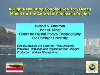
A High Resolution Coupled Sea-Ice/Ocean Model for the Antarctic Peninsula Region. Michael S. Dinniman John M. Klinck Center for Coastal Physical Oceanography Old Dominion University

E N D
A High Resolution Coupled Sea-Ice/Ocean Model for the Antarctic Peninsula Region Michael S. Dinniman John M. Klinck Center for Coastal Physical Oceanography Old Dominion University See also (poster this evening): West Antarctic Peninsula Circulation and Implications for Biological Production: Andrea Piñones et al.
Outline of Presentation • Introduction and Model Description • Ice Shelf Modeling • Sea Ice Modeling • Cross-shelf Transport • Future plans • Conclusions
Research Questions • What is the magnitude and extent of cross-shelf exchange? • What is the structure of the circulation on the WAP shelf? • What are the circulation dynamics that drive the coastal current? • Which physical processes are responsible for exchanges across the permanent pycnocline? • What processes control sea ice in the region? What do we need in a circ. model to help answer?
Antarctic Peninsula Model • ROMS: 4 km horizontal resolution, 24 levels • Ice shelves (mechanical and thermodynamic) • Imposed sea ice or dynamic sea ice model • Bathymetry: ETOPO2v2 + WHOI SOGLOBEC region + Padman grid+ BEDMAP + Maslanyj • Open boundaries: T + S set to SODA, barotropic V relaxed to SODA, baroclinic V pure radiation • Daily wind forcing from a blend of QSCAT data and NCEP reanalyses or Antarctic Mesoscale Prediction System (AMPS) winds • Other atmospheric parameters from several sources (including AMPS)
Ice Shelf Modeling • Ice Shelf basal melt can add large amounts of freshwater to the system (George VI estimated basal melt: 2-5 m/yr) • Ice Shelf does not change in time in model • Three equation viscous sub-layer model for heat and salt fluxes (Holland and Jenkins 1999) • PGF calculation assumes the ice shelf has no flexural rigidity and pressure at the base comes from the floating ice
Model average velocity (net through flow: 0.09 Sv.) Potter and Paren (top,1985) and Jenkins and Jacobs (bottom, 2008, net S to N through flow 0.17-0.27 Sv.)
Sea Ice Modeling • Budgell (2005) model (built into ROMS) • - Thermodynamics based on Mellor and Kantha (1989) with two ice layers, a snow layer, surface melt ponds and a molecular sub layer at the ice/ocean interface • - Dynamics based on an elastic-viscous-plastic rheology after Hunke and Dukowicz (1997) and Hunke (2001) • Los Alamos CICE available, but not using yet due to time constraints
January 2001 January 2002 model ice concentration SSM/I ice concentration
Maximum temperature below 200 m from observations. Klinck et al., 2004 Trajectories of model floats released along the shelf break to show cross- shelf exchange. Piñones et al., poster this evening
Future Plans • Validation of this model • 1 km nested model in MB • CICE sea ice model? • Bathymetry: new Smith and Sandwell, other updates? • Different atmospheric forcing experiments • Lower trophic level ecosystem model
Conclusions • Model is still a work in progress • Several model features appear to be working well - George VI Ice Shelf and supply of fresh water to Marguerite Bay - Sea ice model and interannual variability of ice concentration • Model should be a useful tool for studying effects of circulation on ecosystems in the region
Acknowledgements • AMPS winds courtesy of John Cassano (U. Colorado) • Computer facilities and support provided by the Center for Coastal Physical Oceanography • Financial support from the U.S. National Science Foundation (ANT-0523172)
Based on Smith and Sandwell (v8.2, only north of 72S) Smith andSandwell (v 9.2)
Much warmer water entering the ice shelf cavity than Ross => Much greater melting: 2.1 m/yr (Potter and Paren, 1985) 2.8 m/yr (Corr et al., 2002) 3.1-4.8 m/yr (Jenkins and Jacobs,2008) Model average basal melt under GVI: 6.2 m/yr Jenkins and Jacobs, 2008
Model average velocity 50m below surface (free surface or ice shelf) Model average velocity 400m below surface (free surface or ice shelf)
AMPS Forcing • Antarctic Mesoscale Prediction System: Quasi-Operational atmospheric forecast system in use for the Antarctic • Currently based on PMM5, but transitioning to WRF • We have an archive of analyses and forecasts from 30km grid for 2001-2005 (but much of our model domain not covered before 11/02)
AMPS winds QSCAT/NCEP winds Model ice concentration: October 2004 SSM/I: October 2004
QSCAT/NCEP winds AMPS winds
AMPS Precipitation (9/03-9/05, m/yr) Xie and Arkin Precipitation (m/yr)
Summer surface velocity Original forcing Summer surface velocity AMPS forcing
AMPS winds QSCAT/NCEP winds Model ice concentration: November 2004 SSM/I: November 2004
AMPS winds QSCAT/NCEP winds Model ice concentration: February 2005 SSM/I: February 2005