Download
1 / 22
220 likes | 242 Views
The Circular Flow of Spending and Income, “Multipliers”, “IS-LM”. Lecture 8. The Circular Flow-- in a closed economy. Excise Taxes. Production of Goods. Spending on Purchases of Goods. Wages, Profits, Rents. Saving. Payroll & Income Tax. The Circular Flow-- in a closed economy.

E N D
The Circular Flow of Spending and Income, “Multipliers”, “IS-LM” Lecture 8
The Circular Flow--in a closed economy Excise Taxes Production of Goods Spending on Purchases of Goods Wages, Profits, Rents Saving Payroll & Income Tax
The Circular Flow--in a closed economy (Solid lines reflect current elements sustaining or diverting (in red boxes) from the circular flow) Excise Taxes Production of Goods Spending on Purchases of Goods Wages, Profits, Rents Saving Payroll & Income Tax (Dotted lines indicate potential later return to circular flow)
The Circular Flow--in an open economy Imported Goods Export Demands Excise Taxes Production of Domestic Goods Spending on Purchases of Goods Wages, Profits, Rents Saving Payroll & Income Tax
The Multiplier • The “Multiplier” represents feedback effects within the circular flow of a change in a previous assumption • Obviously, feedback effects are greater the less leakagethere is in the circular flow
The “IS” Curve • The IS Curve is the name given equilibrium set of points denoting • total spending “GDP” corresponding to each interest rate “r”, • for any given fiscal policy and international setting • GDP = C+I+X-M +G • = GDP ( G, T, r, GDPW )
The “IS” Curve (Investment&Saving) • Spending Identity: GDP=C+I+G+X-M (All GDP Output Must be Classified as Some Type of Final Demand) • Income Identity: GDP=C+S +T (All Income that is not Spent on Consumption or paid in Taxes is Saved) • C is common to both, thus I+G+X-M = S + T • or I = S + (T-G) +(M-X) that is, all investment must be financed by personal saving (S), government saving (T-G, the budget surplus), or international borrowing (M-X, also called the international trade or current account deficit) • Assume for simplicity that the last two terms (the government budget and international transactions) are in balance, thus I must = S for the economy to be in balance. The equation summarizing the conditions of income (GDP) and interest rates that will produce such balance is called the IS curve, to reflect the need for I=S, given balance elsewhere.
Why Does the IS Equilibrium Curve Slope Down, with High GDP Paired with Low i, and Vice Versa? • It’s traditional to think of I (investment ) as being negatively correlated with interest rates and S (personal saving) as being positively correlated with GDP (income). Therefore high levels of GDP will produce high levels of saving . If investment demand is to be strong enough to match the saving, then interest rates must be low. And vice versa. • Note from the preceding algebraic derivation that if I (like S) also depends on GDP, and that S (like I) also depends on r, the slope of the IS curve is affected.
The “LM” Curve • Previously, we described interest rates as being a policy decision made by the Federal Reserve in reaction to the level of economy activity : i = f ( GDP). How they achieved this by manipulating reserves and money was implicit in the function. • We could go behind this to look at private demand for money as a function of interest rates and income : the LM Curve
The “LM” Curve • Private demand for money as a function of interest rates and income : the LM Curve • Define “Money” and its portfolio alternatives • Motivations to hold money • Motivations to hold bonds, stocks, durable goods • Combine to motivate demand for money: • Positively correlated with spending • Negatively correlated with interest rates
The “LM” Curve • Solve M/p= Liquidity =f( i , GDP) for i • Plot it in 2 dimensions ( i vs GDP ) for any given level of M/p • This is the “LM” Curve showing points of equilibrium (Liquidity Demanded = Money Supply): • For a given M/p, higher GDP encourages money holding, thus equilibrium requires a higher i to discourage/offset the GDP stimulus
Private Motivation to Hold Money • Keynes’: current transactions, precautionary (possible future transactions), speculative (maximizing return on all assets in uncertain world) • Zero sum game: your incomeandaccumulated wealth in by the end of each period must be consumed or saved; if saved, a form of saving must be chosen • Your choice of “money” as the savings vehicle is a choice against all other options, and is made on the basis of relative tangible and intangible yields and their risks.
Why Is There Such a Focus on “Money?” Rather Than Other Assets? • 1. Tradition: it was originally distinctive because it paid no tangible yield and was the only “perfectly liquid” asset. • 2. The central bank was thought to have greater control over its supply.
Precautionary Demand • Demand to meet emergencies or other needs for large purchases where liquidity is an advantage? • How do you think these would relate to Y, i ?
Speculative Demand • A desire to hold money even with a known low nominal return and only the risk of inflation, versus other financial assets that have capital risk(due to changing interest rates) as well, or versus real goods that are illiquid/ expensive to sell to raise funds. • Explain capital risk on bonds: why the price varies with the market rate after original issue. • Explain risk-return tradeoff. • Ask and explain how speculative demand would relate to income, and to interest rates.
The “LM” Curve • For a given M/p, higher GDP encourages money holding, thus equilibrium requires a higher i to discourage/offset the GDP stimulus i = Interest Rate • i =L( M/p, GDP ) GDP = National Spending or Output
The “LM” Curve is a Hidden Piece of the First Model • Private Demand for Money • M/p (real demand) = f ( i , GDP) • or, i = f ( M/p , GDP ) • The Fed Reactions • Central Bank Supply of Money • M/p = g ( GDP) • If Demand=Supply= ( M / p ) • Then, i = f ( g(GDP) , GDP) = f ( GDP ), the Fed reaction function of the First Model
Elementary Monetarism • velocity=v=nominal GDP/M • nominal GDP= P * realGDP (“Y”) • thus v= P * Y / M • or M * v = P * Y (or sometimes presented as real transactions), known as the quantity equation, the core of the quantity theory of money, whose key conclusion is P = M *(Y/v) and strict monetarism asserts Y, v are fixed in equilibrium • but velocity is not fixed; rather it is sensitive to interest rates
The Velocity of Money (M1) vs. the Treasury Bill Rate Innovations => Rising Velocity
Full Equibrium in both Goods and Money Markets: The “IS-LM” Curves’ Intersection • LM slopes upward: for a given M/p, higher GDP encourages money holding, thus equilibrium requires a higher i to discourage/offset the GDP stimulus • IS slopes downward: higher GDP encourages higher saving, thus equilibrium requires a lower i to encourage Investment i = Interest Rate i =L( M/p, GDP ) GDP = f( i , G, T , GDPW) Equil. i Equil. GDP GDP = National Spending or Output