Download

1 / 20
200 likes | 438 Views
The Circular Flow of Spending and Income, “Multipliers”, “IS-LM. Lecture 7. The Circular Flow-- in a closed economy. Excise Taxes. Production of Goods. Spending on Purchases of Goods. Wages, Profits, Rents. Saving. Payroll & Income Tax. The Circular Flow-- in a closed economy.

E N D
The Circular Flow of Spending and Income, “Multipliers”, “IS-LM Lecture 7
The Circular Flow--in a closed economy Excise Taxes Production of Goods Spending on Purchases of Goods Wages, Profits, Rents Saving Payroll & Income Tax
The Circular Flow--in a closed economy Excise Taxes Production of Goods Spending on Purchases of Goods Wages, Profits, Rents Saving Payroll & Income Tax
The Circular Flow--in an open economy Imported Goods Export Demands Excise Taxes Production of Domestic Goods Spending on Purchases of Goods Wages, Profits, Rents Saving Payroll & Income Tax
The Multiplier • The “Multiplier” represents feedback effects within the circular flow of a change in a previous assumption • Obviously, feedback effects are greater the less leakagethere is in the circular flow
The “IS” Curve • The IS Curve is the name given equilibrium set of points denoting • total spending corresponding to each interest rate, • for any given fiscal policy and international setting • GNP = C+I+X-M +G • = GNP ( G, T, i, GNPW )
The Reduced Forms of the 7 Behavioral Equations • C=C ( G, T, i, GNPW ) • I = I ( G, T, i, GNPW ) • M = M ( G, T, i, GNPW ) • X = X ( G, T, i, GNPW ) • GNP = C+I+X-M +G • = GNP ( G, T, i, GNPW ) • YD = GNP - T • RP = RP ( GNP) = RP( G, T, i, GNPW )
The GNP Reduced Form Equation is a Useful Summary • GNP = C+I+X-M +G= GNP ( G, T, i, GNPW ) • Solve it for GNP=f(i) in 2 dimensions • yields the IS curve GNP1= GNP(G1,T1) i= INTEREST RATE GNP2= GNP(G2,T1) GNP=NATIONAL SPENDING/OUTPUT
The “LM” Curve • Previously, we described interest rates as being a policy decision made by the Federal Reserve in reaction to the level of economy activity : i = f ( GNP). How they achieved this by manipulating reserves and money was implicit in the function. • We could go behind this to look at private demand for money as a function of interest rates and income : the LM Curve
The “LM” Curve • Private demand for money as a function of interest rates and income : the LM Curve • Define “Money” and its portfolio alternatives • Motivations to hold money • Motivations to hold bonds, stocks, durable goods • Combine to motivate demand for money: • Positively correlated with spending • Negatively correlated with interest rates
The “LM” Curve • Solve M/p= Liquidity =f( i , GNP) for i • Plot it in 2 dimensions ( i vs GNP ) for any given level of M/p • This is the “LM” Curve showing points of equilibrium (Liquidity Demanded = Money Supply): • For a given M/p, higher GNP encourages money holding, thus equilibrium requires a higher i to discourage/offset the GNP stimulus
Private Motivation to Hold Money • Keynes’: current transactions, precautionary (possible future transactions), speculative (maximizing return on all assets in uncertain world) • Zero sum game: your incomeandaccumulated wealth in by the end of each period must be consumed or saved; if saved, a form of saving must be chosen • Your choice of “money” as the savings vehicle is a choice against all other options, and is made on the basis of relative tangible and intangible yields and their risks.
Why Is There Such a Focus on “Money?” Rather Than Other Assets? • 1. Tradition: it was originally distinctive because it paid no tangible yield and was the only “perfectly liquid” asset. • 2. The central bank was thought to have greater control over its supply.
Transactions demand • Classic Tobin-Baumol model • per capita M=sq rt (tc*per cap inc / 2i) • M=N * sq rt (tc* Y / N / 2i) • log(M)= .5* (log(N)+log(Y) +log(tc) -log(i)) - log(2) • Be careful about defining Y, the spending measure for private holding: it’s not GNP. Why? • Remember this is only the transactions demand component. Note consensus long-run spending elasticity is close to 1.
Precautionary Demand • Demand to meet emergencies or other needs for large purchases where liquidity is an advantage? • How do you think these would relate to Y, i ?
Speculative Demand • A desire to hold money even with a known low nominal return and only the risk of inflation, versus other financial assets that have capital risk(due to changing interest rates) as well, or versus real goods that are illiquid/ expensive to sell to raise funds. • Explain capital risk on bonds: why the price varies with the market rate after original issue. • Explain risk-return tradeoff. • Ask and explain how speculative demand would relate to income, and to interest rates.
The “LM” Curve • For a given M/p, higher GNP encourages money holding, thus equilibrium requires a higher i to discourage/offset the GNP stimulus i = Interest Rate • i =L( M/p, GNP ) GNP = National Spending / Output
The “LM” Curve is a Hidden Piece of the First Model • Private Demand for Money • M/p (real demand) = f ( i , GNP) • or, i = f ( M/p , GNP ) • The Fed Reactions • Central Bank Supply of Money • M/p = g ( GNP) • If Demand=Supply= ( M / p ) • Then, i = f ( g(GNP) , GNP) = f ( GNP ), the Fed reaction function of the First Model
Elementary Monetarism • velocity=GNP/M1 • GNP=P * T(Real Transactions) • thus v=P * V / M • or M * v = P * T, known as the quantity equation, the core of the quantity theory of money, whose key conclusion is P = M *(Y/v) and strict monetarism asserts Y, v are fixed in equilibrium • but velocity is not fixed; rather it is sensitive to interest rates
The Velocity of Money (M1) vs. the Treasury Bill Rate (percent) (GDP/M1)