Download
1 / 43
430 likes | 528 Views
This research focuses on motion estimation of plant root growth using advanced image processing techniques. The study aims to provide higher spatial and temporal accuracy in root growth profiling. The methods utilized include differential, correlation-based, frequency-based, and probability-based techniques. Key contributions include an easy-to-use software package for root growth estimation and a novel framework for dealing with non-uniform deformable motions. The tensor-based method offers advantages such as simultaneous segmentation and motion estimation, but is limited to low-motion scenarios and is sensitive to noise.

E N D
Robust Tensor-based Velocity Estimation of Plant Root Growth M. S. Degree presentation Hai Jiang Advisor K. Palaniappan Computer Engineering & Computer Science Department University of Missouri - Columbia
Motivation • Biological applications demand estimating the plant root growth with high accuracy [Beemster, 1998]. The objective is to generate a growth profile from the root tip along the root. In the computer vision sense, this is motion estimation from image sequences. • The following plant root was mosaiced from the center frames of 10 segments. The size of each segment image sequence is 640pix*480pix*9 frame, and 1 pixel=0.885um.
Motivation • The application of existing motion estimation methods on this plant root data is not straightforward and the users need to adjust a lot of parameters to fulfill the task. • This research work was encouraged by the success of the estimation of plant leaf growth by the group of Bernd Jahne in Univ. of Heidelberg, Germany[Schmundt, 1995]. • This research work is valuable for other biological motion estimation applications.
Contribution • Novel work and successful experiences in motion estimation of plant root growth using image processing techniques. • Higher spatial and temporal accuracy, faster motion extraction than traditional numerical work. Developed an easy-to-use software package to do root growth estimation. • A novel framework in dealing with non-uniform deformable motions. Knowledge acquired in this work will be useful in extracting aerospace dynamic analysis and flux computation in the sea or rivers.
Popular Methods • Differential methods • Correlation-based methods • Frequency-based methods • Probability-based methods
Differential Methods • Constant illumination assumption • Optical flow equation Ixvx + Iyvy + It= 0 • The tensor-based method is an extension of optical flow method
Correlation-based Methods • Based on region similarity, easy to adjust • Max-convolution or Min-squared error • Robust functions • Computation intensity problem • Local deformation problem
Frequency-based Methods • Correspondence of motion and lines/planes in frequency domain • Phase-based methods • Easy to find motions with regular patterns • Hard to deal with normal motions
Probability-based Methods • Maximization of the possibilities of plans of reconstructing the previous images using pixels in the later images • Bayesian methods, EM methods, annealing • Ability to deal with occlusions and deformations
Robust Matching Method • Minimization of the cost function • + • Where Frame at time t1 Frame at time t2 N l w Searching domain D L W N’ matching
Robust Matching Method • Confidence Tests • Statistical confidence test. • e.g. threshold on ||AVG(Cost)-MIN(Cost)||/STD_VAR(Cost) • Forward-backward consistency test Image at time t Image at time t+ t M s s’’ s’ M
The Problem of Robust Matching • Segmentation not uniform for matching methods: • The anisotropy of the tensor indicates if there is motion or not. e.g. threshold on the coherency. • Computation intensity: about one hour to analyze one sequence of 9 frames of size 640x480 using robust matching algorithm.
Image Volume • A moving point forms a line in the volume • A moving edge forms a plane in the volume • Under constant illumination assumption, the trace of a moving point is a line with constant intensity y y x t t
The Tensor-based Method • In the image volume, we have • That means the motion estimation can be done by estimating the orientations of the constant lines inside the image volume. Image volume y axis Constant gray level line (The bold line) x t t axis x axis
The Tensor-based Method • The orientation of iso-gray value lines within a 3D spatiotemporal neighborhood U can mathematically be formulated [Jahne, as the direction nbeing as much perpendicular to all gray value gradients g in U as possible, i. e. • This can be formulized as and • where
The Tensor-based Method • The 3D structure tensor for x-y-t image volume has the structure • J = • It can be shown that this expression is minimized if the vector nis given by the eigenvector of the tensor J to the minimum eigenvalue.
The Tensor-based Method Eigen Analysis of the tensor
The Tensor-based Method • Velocity computation • For rank 1: • For rank 2: • For rank 0, v=0 • For rank 3, no motion can be extracted
The Tensor-based Method • Advantages • Simultaneous segmentation and motion estimation • Uniform computation framework • Faster than robust matching method • The problems: • Velocity extraction is limited to rank 0, 1, and 2 • Only suitable for low-motion estimation (see following figure) • Very sensitive to noises • Aperture problem Trace of slow motion local neighborhood image sequence Trace of fast motion t
Robust Tensor Method • A new framework has been proposed in the thesis work. It is the combination of the tensor method and the robust matching method. • The idea is doing the tensor-based method followed by the robust matching method. The robust matching method takes advantage of the segmentation of the tensor method, uses the velocity values computed by the tensor method to initialize the start value of its velocity, and construct a much smaller searching domain. Searching Domain Local Window P Original site s H | L | Initial v Final v
Robust Tensor Method Original Image Sequence Preprocessing: Filtering and Illumination Calibration The pure tensor method Optimal Filter Computation Compute Tensor Field Using ‘coherency’ to compute segmentation mask Compute approximate velocity using tensor method The robust matching method Use the velocity results from the tensor method to initialize the robust matching searching domain. Only compute the velocity for the sites inside the segmentation mask. Statistical confidence test is done here. Compute both the forward matching and the backward matching. Confidence Tests (Forward-backward Matching Consistence test) interpolate the velocity field
Robust Tensor Method • Preprocessing • Using Gaussian smooth filter to remove high frequency noises. • Do illumination calibration for each frame in the image sequence • Pav = 0; • Read in the image sequence in DD[][][], which should contains tensorsize+2 frames • For t = 1 to tensorsize+2 do • Initialize Av[t] = 0; • For each pixel in the frame DD[t][][] do • Av[t] = Av[t] + DD[t][i][j]; • Pav = Pav + Av[t]; • Pav = Pav / (tensorsize+2); • For t=1 to (tensorsize+2) do • For each pixel in DD[][][] • DD[t][I][j] = DD[t][i][j] + (Pav – Av[t])/(area of a frame);
Robust Tensor Method • Optimal filter and derivative computation in x-y-t space • Optimal filters are used to compute derivatives which is invariant to the orientation of the coordinates • 3D optimal sobel filter • (1 0 -1) x = (1 0 –1) x (A) • = • Derivatives are computed by convolving the sobel filters with the intensity in the local 3D neighborhood
Robust Tensor Method • Interpolation • Assign a pixel x’ inside the holes with the weighted average over the local neighborhood N: • where W(x-x’) is a weighting function which post more weights on pixels close to x’, and less weights on distance pixels. Gaussian normal function can be one good choice.
Robust Tensor Method A C B
Robust Tensor Method D F E
Robust Tensor Method G H vx vy
Velocity Profile Mosaicing • To mosaic profiles of each root segment, kinetic mosaicing is needed. • The problem is when imaging later segments, the previous segments are still growing. The whole velocity profile can not be generated by directly concatenate each segment profile. • The referring coordinates are chosen to be the background, and assume the growth speed is constant to time for one segment. So the solution is first find the motion of camera by finding the registration information of the background images, then directly put the profile in the right place. Vertical lifting is done if the overlapping curves are not jointed. For details please read chapter 7 on my thesis.
Designed Experiments • To find the optimal frame-displacement range • To find best tensor size • To estimate effects of time on the growth speed • Correctness verification
Experiment to find the optimal frame-displacement range Suitable displacement range is found to be 0.4~2.8 pixels/frame, and the optimal velocity to estimate with lowest error is 2.2 pixels/frame.
Experiments to find the optimal tensor size Note: The tensor size is PxPxP, P=2r+1. The horizontal axis stands for r.
Experiment to extract the profile of tip velocity over time • Find the tip region by first segmenting the root using tensor method • Run the robust tensor algorithm on the tip region, extract the average/median velocity of the tip region • The estimation of the tip region of the next stack can be calculated from the tip velocity currently computed.
V, V (pix/fr) Method X Direction Y Direction Motion Field Density (%) Error Rate (%) Mean (pix/fr) Std.Var. (pix/fr) Mean (pix/fr) Std.Var. (pix/fr) V =0.0 V =0.0 Pure tensor 0.000000 0.000000 0.000000 0.000000 96.8340 0.000000 Robust tensor 0.000000 0.000000 0.000000 0.000000 99.6133 0.000000 V =0.0 V =1.0 Pure tensor 0.367220 0.180056 1.073452 0.110630 48.9141 13.45243 Robust tensor 0.000000 0.000000 1.000000 0.000000 99.0161 0.000000 V =1.0 V =0.0 Pure tensor 1.029664 0.071725 0.219483 0.225242 48.6139 5.279663 Robust tensor 1.000000 0.000000 0.000000 0.000000 99.1329 0.000000 V =1.0 V =1.0 Pure tensor 0.978694 0.270083 0.950715 0.254160 96.9147 3.519407 Robust tensor 1.000000 0.000000 1.000000 0.000000 98.4884 0.000000 Correctness Verification • The robust tensor algorithm has been tested on synthetic root sequences, and high accuracy is achieved.
Profile Mosaiced for the Whole Root Biological scientists can make derivative over the distance from the tip on this curve and find the growth rate of each part of the plant root.
Summary • By combining the tensor method and the robust matching method, this thesis work has provided a novel framework to estimate non-uniform small deformable motions. • A software package to automatically estimate the spatio-variant growth profile of plant roots and the tip velocity profile over time is developed. • This work was done on SGI Octane with R10k 195M Hz Mips CPU and 512M main memory.
Future Research Work • Algorithm competition with other popular motion estimation methods • Parameter normalization of this algorithm to adapt various image sequences • Better approaches of tip velocity tracking over time. • Refine the model of tensor method to reduce the error of tensor method • Try to implement a fast searching algorithm for the minimum in the robust matching method. • Theory work of tensor method, about the problems of motion dis-/occlusion, local deformations, illumination changing. Explore the possibility to estimate the velocity for those motions when the tensor is not in rank 0, 1 or 2. • Intension of combining the tensor method with probability-based motion estimation methods.
References • G.T.S. Beemster and T.I. Baskin, Analysis of Cell Division and Elongation Underlying the Develop-mental Acceleration of Root Growth in Arabidopsis thealiana L., Plant Physiology (1998). • D. Schmundt, M. Stitt, B. Jahne and U. Schurr, Quantitative analysis of the local rates of growth of dicot leaves at a high temporal and spatial resolution, The Plant Journal(1998) 16(4), 505-514. • S.S. Beauchemin and J. L. Barron, The computation of optical flow, ACM Computing Surveys(1995), Vol. 27, No. 3. • H. HauBecker and B. Jahne, A Tensor Approach for Precise Computation of Dense Displacement Vector Fields, Proc. Mustererkennung 1997, Braunschweig, 15-17, Informatik Aktuell, Springer, Berlin, 199-208. • H. Knutsson and C-F. Westin. Normalized and Di_erential Convolution: Methods for Interpolation and Filtering of Incomplete and Uncertain Data. In Proceedings of IEEE Computer Society Conference on Computer Vision and Pattern Recognition, pages 515{523, New York City, USA, June 1993.
References • 6. H. Knutsson, C-F. Westin, and C-J. Westelius. Filtering of Uncertain Irregularly Sampled Multidimensional Data. In Twenty-seventh Asilomar Conf. On Signals, Systems & Computers, pages 1301{1309, Paci_c Grove, California, USA, November 1993. IEEE • G. Farneback, Spatial Domain Methods for Orientation and Velocity Estimation, LIU-TEK-LIC-1999:13, Dept. of E. E., Linkopings Univ., 1999, ISBN 91-7219-441-3, ISSN 0280-7971. • S.S. Beauchemin and J.L. Barron, The Computation of Optical Flow, ACM Comp. Surveys, Vol. 27, No.3, 1995.
References • 9 J. L. Barron, D. J. Fleet, and S. S. Beauchemin, Performance of optical flow techniques. Technical Report RPL-TR-9107, Queen’s University, Kingston, Ontario, Robotics and Perception Laboratory Technical Report, July 1992. • 10. Eero P. Simoncelli, Design of Multi-Dimensional Derivative Filters, First IEEE Int'l Conf. on Image Proc., Austin TX, Nov. 1994. • 11. Hany Farid and Eero P. Simoncelli, Optimally Rotation-Equivariant Directional Derivative Kernels, 7th Int'l Conf. Computer Analysis of Images and Patterns, Kiel, Germany, Sept. 10-12, 1997.
References • H. HauBecker and B. Jahne, A Tensor Approach for Precise Computation of Dense Displacement Vector Fields, Proc. Mustererkennung 1997, Braunschweig, 15-17, September 1997, Informatik Aktuell, Springer, Berlin, 199-208. • Ye, M.; Haralick, R.M., Optical flow from a least-trimmed squares based adaptive approach, Pattern Recognition, 2000. Proceedings. 15th International Conference on Volume: 3 , 2000 Page(s): 1052 -1055 vol.3. • 14. Ye, M.; Haralick, R.M., Two-stage robust optical flow estimation, Computer Vision and Pattern Recognition, 2000. Proceedings. IEEE Conference on , Volume: 2 , 2000, Page(s): 623 -628 vol.2.