Download
1 / 12
120 likes | 267 Views
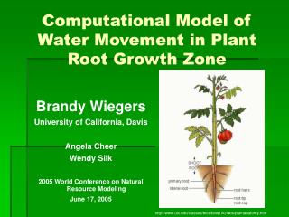
This material is based upon work supported by the National Science Foundation under Grant #DMS-0135345. Brandy Wiegers University of California, Davis. 3D Computational Model of Water Movement in Plant Root Growth Zone. Under the Direction of Dr. Angela Cheer

E N D
This material is based upon work supported by the National Science Foundation under Grant #DMS-0135345 Brandy Wiegers University of California, Davis 3D Computational Model of Water Movement in Plant Root Growth Zone Under the Direction of Dr. Angela Cheer email: wiegers@math.ucdavis.edu website: http://math.ucdavis.edu/~wiegers
Relationship between growth and water potential L(z) = ▼·(K·▼) (1) • Notation: • Kx, Ky, Kz: The hydraulic conductivities • fx = f/x • In 3D: L(z) = Kxxx+ Kyyy +Kzzz+ Kxxx KyyyKzzz (3)
zmax rmax Model Assumptions Model Setup Boundary Conditions (Ω) • The tissue is cylindrical, with radius x, growing only in the direction of the long axis z • = 0 on Ω • Corresponds to growth of root in pure water • Δr = Δz = 0.1 mm • rmax = 0.5 mm • Zmax = 10 mm • Osmotic Model: The distribution of is axially symmetric. Source Model: This assumption no longer holds. Look at the phloem structure. It’s not regularly distributed. Add a set of distributed sources within the radial cross-section of the root. • The growth pattern does not change in time. • Conductivities in the radial (Kx) and longitudinal (Kz) directions are independent so radial flow is not modified by longitudinal flow. 2D Visualization of 3D Resulting Models Experimental Data Osmotic Model Known Values: L(z), Kx,Ky, Kz, on Ω Source Model Known Values: L(z), Kx,Ky, Kz, on Ω and at source cells. L(z) = Kxxx+Kyyy+Kzzz+Kxxx+Kyyy+Kzzz (3) = f(Kξξ,Kηη,Kζζ,ξ,η,ζ,ξξ,ηη,ζζ,ξη ,ξζ,ηζ) L = [Coeff] , Solve matrix equation for • Kx, Kz : 4 x10⁻⁸cm2s-1bar-1 - 8 x10⁻⁸cm2s-1bar-1 • L(z) : 1/hr
The Research Problem Motivation Primary plant root growth is dependent on water movement within the growth zone. Thus, an understanding of plant root growth can be helpful in understanding crop draught and other water-soil-plant interactions. • 1980: Silk and Wagner created the Osmotic Root Growth Model, which predicated a radial water potential gradient in the plant root growth zone. • 2004: Laboratory techniques/ equipment was finally available to be able to test this hypothesis. Empirical evidence did not support the 1980 theory. • 2004: Gould, et al find evidence that phloem is extending into the plant root growth zone. History of the Problem Problem Statement It is our hypothesis that the phloem sieve cells that extend into the primary plant root growth zone provide a water source to facilitate the plant root growth process. This hypothesis is tested using a computational model of the plant root growth zone water potential. Gould, et al 2004
Generalized Coordinates Fletcher, 1991 Applying Generalized Coordinates to (3) L(z) = Kxxx+Kyyy+Kzzz+Kxxx+Kyyy+Kzzz (3) Kxx = Kxξξx +Kxηηx + Kxζζx x = /x= ξξx +ηηx + ζζx xx = (x)x = (x)ξξx + (x)ηηx + (x)ζζx = (ξξx +ηηx + ζζx)ξξx + (ξξx +ηηx + ζζx)ηηx + (ξξx +ηηx + ζζx)ζζx Converts any grid (x,y,z) into a nice orthogonal grid (ξ,η,ζ) using Jacobian (J) and Inverse Jacobian (J-1)
Osmotic Model Results : Growth Sustaining Water Potential Analysisof Results This Model predicts: • Radial and Longitudinal gradient Laboratory Tests Have Shown: • No radial gradient • Longitudinal gradient does exist THE OSMOTIC MODEL PREDICTED RADIAL GRADIENT CAN NOT BE PROVEN IN A LABRATORY
Zone of Maturation Zone of Elongation Sieve Tube Zone of Cell Division Apical Meristem Root Cap Plant Physiology Growth Zone Anatomy Plant Cell Growth Expansive growth of plant cells is controlled principally by processes that loosen the wall and enable it to expand irreversibly(Cosgrove, 1993). Plant Cell Water Facilitated Cell Growth http://www.troy.k12.ny.us/faculty/smithda/Media/Gen.%20Plant%20Cell%20Quiz.jpg http://sd67.bc.ca/teachers/northcote/biology12/G/G1TOG8.html Rules of Plant Cell Growth • Water must be brought into the cell to facilitate the growth (an external water source). • The tough polymeric wall maintains the shape. • Cells must shear to create the needed additional surface area. • The growth process is irreversible
Numerical Methods η ξ 2nd Order Finite Difference Approximations Given general function G(i,j): • G(i,j)ξ = [G(i+1,j)–G(i-1,j) ] / (2Δξ) + O(Δξ2) • G(i,j)ξξ = [G(i+1,j) -2G(i,j)+ G(i-1,j)] / (Δξ2) + O(Δξ2) • G(i,j)ξη = [G(i+1,j+1) -G(i-1,j+1)–G(i+1,j-1) + G(i-1,j-1) ] / (4ΔξΔη) + O(ΔξΔη)
Source Model Results : Growth Sustaining Water Potential Analysisof Results This Model predicts: • Decreased Radial and Longitudinal gradient THE CURRENT SOURCE MODEL PREDICTION OF REDUCED RADIAL GRADIENT IS REASONABLE IN TERMS OF THE LABORATORY EXPERIMENTATION THE MODEL NEEDS TO BE FURTHER DEVELOPED
Growth Variables Hydraulic Conductivity (K) Water Potential () • wgradient is the driving force in water movement. • w = s + p + m • Gradients in plants cause an inflow of water from the soil into the roots and to the transpiring surfaces in the leaves (Steudle, 2001). • Measure of ability of water to move through the plant • Inversely proportional to the resistance of an individual cell to water influx • Typical values: Kr ,Kz = 8 x 10⁻⁸ cm2s-1bar-1 http://www.soils.umn.edu/academics/ classes/soil2125/doc/s7chp3.htm Relative Elemental Growth Rate (L) • A measure of the spatial distribution of growth within the root organ. Measured using a marked growth experiment. • Co-moving reference frame centered at root tip. • L(z) = lim(AB→0)(1/(AB) [V(A)- V(B)]) • Generalize this as: L(z) = ▼ · g Erickson and Silk, 1980
Generalized 2-d Coordinate Discretization L(z) = (i+1,j) (Cξ/(2Δξ)+Cξξ/(Δξ)2 ) + (i-1,j) (-Cξ/(2Δξ)+Cξξ/(Δξ)2 ) + (i,j+1) (Cη/(2Δη)+ Cηη/(Δη)2 ) + (i,j-1) (-Cη/(2Δη)+ Cηη/(Δη)2 ) - 2 (i,j) (Cξξ/(Δξ)2 + Cηη/(Δη)2 ) +(i+1,j+1) Cξη/(4ΔξΔη) - (i-1,j+1) Cξη/(4ΔξΔη) - (i+1,j-1) Cξη/(4ΔξΔη) + (i-1,j-1) Cξη/(4ΔξΔη) L = [Coeff]
End Goal… Future Work… • Continued Work on Root Grid: Refinement and Generation • Modification of Source Water Potential Phloem contains many dissolved solutes, Use ≠ 0 for the source terms. • Looking at different plants This work is done with a corn model, other plants need to be examined Computational 3-d box of soil in which the plant roots grow in real time while changes in growth variables are monitored.