迴歸分析 Regression Analysis
迴歸分析 Regression Analysis. 簡單迴歸與多元迴歸 Simple and Multiple regression. 基本定義 簡單迴歸:以單一自變項去解釋(預測)依變項的迴歸分析 多元迴歸:同時以多個自變項去解釋(預測)依變項的迴歸分析 各變項均為連續性變項,或是可為虛擬為連續性變項者 方程式 簡單迴歸: Y=b 1 x 1 +a 多元迴歸: Y=b 1 x 1 +b 2 x 2 +b 3 x 3 +……+b n x n +a 多元迴歸的特性: 對於依變項的解釋與預測,可以據以建立一個完整的模型。

迴歸分析 Regression Analysis
E N D
Presentation Transcript
迴歸分析 Regression Analysis
簡單迴歸與多元迴歸Simple and Multiple regression • 基本定義 • 簡單迴歸:以單一自變項去解釋(預測)依變項的迴歸分析 • 多元迴歸:同時以多個自變項去解釋(預測)依變項的迴歸分析 • 各變項均為連續性變項,或是可為虛擬為連續性變項者 • 方程式 • 簡單迴歸:Y=b1x1+a • 多元迴歸:Y=b1x1+b2x2+b3x3+……+bnxn+a • 多元迴歸的特性: • 對於依變項的解釋與預測,可以據以建立一個完整的模型。 • 各自變項之間概念上具有獨立性,但是數學上可能是非直交(具有相關) • 自變項間的相關對於迴歸結果具有關鍵性的影響。
誤差 迴歸離均差 原始離均差 Xi 迴歸分析的統計原理:變異數拆解與F test • 利用回歸方程式,依變項Y變異量當中可以被解釋的部分稱為回歸變異量 • 無法被解釋的部分稱為殘差變異量 • SSy=SSreg+SSres
迴歸可解釋變異量比(R2) • 迴歸可解釋變異量比,又稱為R2(R square),表示使用X去預測Y時的預測釋力,即Y變項被自變項所解釋的比率。反應了由自變項與依變項所形成的線性迴歸模式的契合度(goodness of fit) • 又稱為迴歸模型的決定係數(coefficient of determination),R2開方後可得multiple R,為自變項與依變項的多元相關。 • 此一數值是否具有統計上的意義,反映了此一迴歸分析或預測力是否具有統計上的意義,必須透過F考驗來判斷
Adjusted R2 • 以樣本統計量推導出來的R2來評估整體模式的解釋力,並進而推論到母群體時,會有高估的傾向 • 樣本數越小,越容易高估,解釋力膨脹效果越明顯,樣本數越大,膨脹情形越輕微 • 校正後R2(adjusted R2),可以減輕因為樣本估計帶來的R2膨脹效果。當樣本數越小,應採用校正後R2。
迴歸係數(regression coefficient) • 迴歸方程式Y=bX+a • B係數: • 為一未標準化的迴歸係數,其意義為每單位X值的變動時,Y所變動的原始量 • B係數適用於實務工作的預測數值的計算 • 係數: • 如果將b值乘以X變項的標準差再除以Y變項的標準差,即可去除單位的影響,並控制兩個變項的分散情形,得到新的數值(Beta),為不具備特定單位的標準化迴歸係數 • 係數也是將X與Y變項所有數值轉換成Z分數後,所計算得到的迴歸方程式的斜率,該方程式通過ZX,ZY的零點,因此截距為0。 • 係數具有與相關係數相似的性質,也就是介於-1至+1之間,其絕對值越大者,表示預測能力越強,正負向則代表X與Y變項的關係方向。 • 係數適用於變項解釋力的比較,偏向學術用途
多元共線性的檢驗 • 對於某一個自變項共線性的檢驗,可以使用容忍值(tolerance)或變異數膨脹因素(variance inflation factor, VIF)來評估。 • Ri2為某一個自變項被其他自變項當作依變項來預測時,該自變項可以被解釋的比例,1- Ri2(容忍值)為該自變項被其他自變項無法解釋的殘差比 • Ri2比例越高,容忍值越小,代表預測變項不可解釋殘差比低,VIF越大,即預測變項迴歸係數的變異數增加,共變性越明顯。 • 整體迴歸模式的共線性診斷可以透過特徵值(eigenvalue)與條件指數(conditional index; CI)來判斷。 • 各變量相對的變異數比例(variance proportions),可看出自變項之間多元共線性的結構特性。當任兩變項在同一個特徵值上的變異數比例接近1時,表示存在共線性組合。
Basic assumptions to regression • Assumptions • Assumptions for residuals (error scores) • Zero Mean • Homoscedastic • Independence with predictors • Normality • Assumptions for specification errors • Linear relationship • All relevant predictors must be included • No irrelevant predictors can be included • Assumptions for measurement errors • Relevant measurement procedures and variable selections • Providence of the goodness index of measurement
Issues in Regression • Multicollinearity • Theoretical issues • Analytic or Technical issues • Measurement issues • Categorical variable as predictors • Effect coding • Dummy coding • Type of regression analysis • Determination of selection procedures of predictors • Simultaneous regression • Stepwise regression • Hierarchical regression • Controlling for Type I and II error • Less is more • Theoretical consideration • Measurement consideration
迴歸的應用模式 • Two applications of correlation and regression • Prediction To predict events or behavior for practical decision-making purposes in applied settings • Explanation To understand or explain the nature of a phenomenon for purpose of testing or developing theories
預測型迴歸 • Determining the predictor variables and criterion variables • Searching for valid variables and removing the unnecessary variables • Deriving a linear formula: multiple regression equation (Usage of derivation study) • Linear equation is custom-made, therefore the accuracy and degree of relationship may shrink among studies • Strategy for shrinkage • Cross-validation study Conducting a second study to evaluate how well the formula form the derivation study actually predicts for other people from the same population • Shrinkage formulas determining the amount of shrinkage by obtain an estimate by means of one of several formulas, correcting for the number of predictors relative to the number of subjects
預測型迴歸的程序 • Multiple regression equation • Partial regression coefficients • Intercept: score of the criterion varible when all of the predictors are zero • Predicted score • Raw score or standard score regression equation • Accuracy of prediction • Multiple correlation coefficient (R) • Coefficient of multiple determination (R2) • Simultaneous or stepwise procedure • Significance test for R2 by ANOVA • Interval estimation (standard error of estimate; SEest) • Standard deviation of the distribution of the error scores • 95% confident interval of predicted scores
解釋型迴歸 • Conceptualization to the differences • The ability to make causative and explanatory interpretations is determined primarily by the design of the data collection and the logic of the reasoning rather than by the procedures for analyzing the data • Including and dropping predictor variables has to be under in both serious theoretical consideration or data analysis procedures • Two main tasks • Identifying those factors with which is co-occurs • Ruling out plausible alternative causal explanations using statistical control instead of experimental control
解釋型迴歸的程序 • Accuracy of explanation • Multiple correlation coefficient (R) • Coefficient of multiple determination (R2) • Significance test for R2 by ANOVA • Independent contribution and statistical control • Correlation coefficients • First-order, partial, part coefficients • Partial regression coefficients • Raw or Standardized coefficients • Relative importance of predictors
多元迴歸的變項選擇程序:II 技術考量:逐步分析法(stepwise multiple regression) • 所有的預測變項並非同時被取用來進行預測,而是依據解釋力的大小,逐步的檢視每一個預測變項的影響,稱為逐步分析法。 • (一)順向進入法(forward) • 預測變項的取用順序,以具有最大預測力且達統計顯著水準的獨變項首先被選用,然後依序納入方程式中,直到所有達顯著的預測變項均被納入迴歸方程式。 • (二)反向淘汰法(backword) • 與順向進入法相反的程序,所有的預測變項先以同時分析法的方式納入迴歸方程式的運算當中,然後逐步的將未達統計顯著水準的預測變項,以最弱、次弱的順序自方程式中予以排除。直到所有未達顯著的預測變項均被淘汰完畢為止。 • (三)逐步分析法(stepwise) • 綜合順向進入法與反向淘汰法,
多元迴歸的變項選擇程序:I 理論考量:同時、階層與路徑 • 同時分析法(simultaneous multiple regression) • 所有的預測變項同時納入迴歸方程式當中。 • (一)強制進入法 • 在某一顯著水準下,將所有對於依變項具有解釋力的預測變項納入迴歸方程式,不考慮預測變數間的關係,計算所有變數的迴歸係數。 • (二)強制淘汰法 • 與強迫進入法相反,強制淘汰法之原理為在某一顯著水準下,將所有對於依變項沒有解釋力的預測變項,不考慮預測變數間的關係,一次全部排除在迴歸方程式之外,再計算所有保留在迴歸方程式中的預測變數的迴歸係數。 • 階層分析法(hierarchical multiple regression) • 預測變項間可能具有特定的先後關係,而需依照研究者的設計,以特定的順序來進行分析。
逐步法與同時法比較 • 逐步分析法較同時進入法可以找到最有預測力的變項,同時也可以避免共線性的影響,適合做探索性的研究使用。 • 逐步法適合用以預測性研究,協助建立最佳預測模型 • 逐步法是以統計程序處理變項重要性,在理論解釋性研究缺乏基礎 • 同時法的優點則是可以從整體效果模式中看到所有自變項的效果,每一個自變項的解釋力皆被考慮與呈現。
模式檢驗 模式摘要 顯示自變項對依變項的整體解釋力。 所有自變項可以解釋依變項95.4%的變異。調整後的R平方為89.6%,因樣本小,宜採校正後的R平方。 模式顯著性整體考驗 用以檢驗整體迴歸模式的顯著性。 F考驗值16.522與p=.009顯示上述89.6%的迴歸解釋力是具有統計意義
參數估計與共線性分析 共線性估計 個別變項預測力的檢驗。允差(即容忍值)越小,VIF越大表示共線性明顯。如期中考成績與其他自變項之共線性嚴重。 整體模式的共線性檢驗 特徵值越小,條件指標越大,表示模式的共線性明顯。 條件指標181.422顯示有嚴重的共線性問題,偏高的變異數比例指出作業分數(.76)、期中考(.80)與期末考成績(.85)之間具有明顯共線性。
殘差分析 檢驗極端值的存在,以及是否違反常態性假設。 殘差為觀察值與預測值的差,殘差越大表示誤差越大,標準化後的殘差絕對值若大於1.96表示為偏離值。 雖無明顯偏離值,但是殘差並非呈現常態分配。(因樣本過少)。
逐步迴歸法 逐步迴歸法自變項進入或刪除清單。與選擇標準。進入以F機率.05,刪除以F機率.10為標準 總計兩個變項分兩個步驟(模式)被選入迴歸方程式。期末考成績與缺席次數。