Download
1 / 65
660 likes | 793 Views
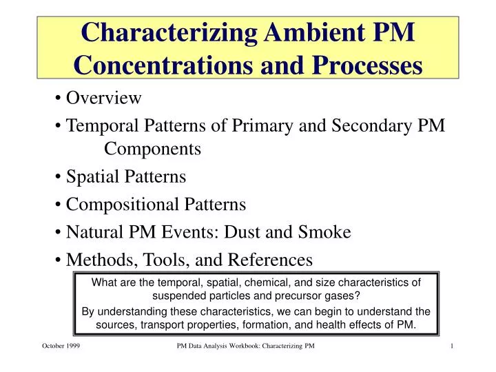
Characterizing Ambient PM Concentrations and Processes. Overview Temporal Patterns of Primary and Secondary PM Components Spatial Patterns Compositional Patterns Natural PM Events: Dust and Smoke Methods, Tools, and References.

E N D
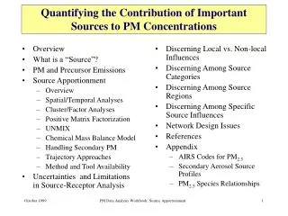
Characterizing Ambient PM Concentrations and Processes • Overview • Temporal Patterns of Primary and Secondary PM Components • Spatial Patterns • Compositional Patterns • Natural PM Events: Dust and Smoke • Methods, Tools, and References What are the temporal, spatial, chemical, and size characteristics of suspended particles and precursor gases? By understanding these characteristics, we can begin to understand the sources, transport properties, formation, and health effects of PM. PM Data Analysis Workbook: Characterizing PM
Overview • Spatial and temporal analyses of PM data are the basis for improving our understanding of emissions and the dynamic atmospheric processes that influence particle formation and distribution. Goals of the data analyst performing these investigations can include: • identifying possible important sources of PM and precursors • determining chemical and physical processes that lead to high PM concentrations • assessing efficacy of existing control strategies • Analyses help one to develop a conceptual model of processes affecting PM concentrations. Questions the analyst could be addressing with the data include the following: • What is the chemical composition of PM and how does the composition change with time and by site? • What are the statistical characteristics of pollutant concentrations and how do they change from site to site and from time to time? • How do different pollutant concentrations vary in space and time relative to each other? • What spatial and temporal scales are represented by pollutant measurements at each site? • What local or regional sources influence a given measurement site? • How did meteorology, nearby precursor and PM emissions, and natural events influence both spatial and temporal characteristics of the PM data? • Many of the more detailed analyses discussed later in this workbook, such as source apportionment, are improved by a thorough understanding of spatial and temporal characteristics. For example, the analyst can point out key features in the data that need to be reproduced in modeling efforts used to assess control strategies or can identify key components of PM for source apportionment. Clearly, spatial and temporal characterization of the data is a fundamental part of all the workbook chapters. Solomon, 1994 PM Data Analysis Workbook: Characterizing PM
Decision Matrix for Spatial and Temporal Analyses Decision matrix to be used to select analysis objectives for the characterization of PM. To use the matrix, find your analysis objective across the top. Follow this column down to see which technical topic areas at the left illustrate analyses pertaining to the objective. For each of these analysis objectives, go to the next page to see which data and data analysis tools might be needed to meet the objective. PM Data Analysis Workbook: Characterizing PM
Decision Matrix for Spatial and Temporal Analyses For each of the analysis objectives that are of interest to you, follow down the column to see which data and data analysis tools might be needed. PM Data Analysis Workbook: Characterizing PM
Temporal Patterns of Primary and Secondary PM Components • Diurnal patterns: explore the daily cycle of PM and its relationship to emissions and meteorology. • Day of week patterns: explore the weekly cycle of PM and its relationship to emissions. • Episodic patterns: explore differences between episodes of high PM concentrations and non-episodes. • Seasonal patterns: explore differences in seasonal PM concentrations and the causal factors. PM Data Analysis Workbook: Characterizing PM
Diurnal Patterns: Overview • Since the ambient PM standard is expressed as a daily average (65 g/m3), most measurements of PM are 24-hr averages. Hourly values are not relevant for regulating compliance purposes. • When measurements with shorter averaging times than 24-hr are available, analysts have observed a significant diurnal pattern of PM at most locations. • The diurnal PM variation is due to the daily cycle of emissions, dispersion, and PM formation and removal processes. • The diurnal variation of PM is not well understood, mostly because of data limitations. However, the limited data can be used to suggest possible influences. PM Data Analysis Workbook: Characterizing PM
Diurnal Pattern of PM in an Urban Setting Figures prepared using Voyager. Note that the PM2.5 and PM10 monitors are sited ~ 1 mile apart. Husar, 1999 In the summer in New Haven, CT, the PM2.5 concentrations are nearly constant throughout the day while the PM10 concentrations peak during the day due to increases in the coarse particle fraction. In the winter, the PM2.5 appears to have small peaks during the rush hours. In contrast, the PM10 concentration doubles during the day due to increases in coarse particle concentrations. PM Data Analysis Workbook: Characterizing PM
Diurnal Pattern of PM in a Rural Setting Husar, 1999 In the summer in Liberty, PA, the PM2.5 and PM10 concentrations peak at night and decrease during the daytime. The daily cycle of nighttime boundary layer formation and daytime mixing height growth appear to drive PM concentrations. In the winter, the PM2.5 and PM10 concentrations show a mild diurnal fluctuation because there is a smaller difference between daytime and nighttime inversion heights. PM Data Analysis Workbook: Characterizing PM
Diurnal Pattern of PM in Southern California Husar, 1999 In Long Beach, CA, the PM10 concentration is low at night and peaks at about 1400 PST, followed by a sharp drop with the arrival of the sea breeze. The sea breeze is composed of relatively clean, cool air that does not mix significantly with the more-polluted mixed layer. At Indio, CA, in the California desert, the PM10 concentration peaks in the afternoon. Is this increase caused by wind-blown dust? By transported PM from the upwind urban area ? PM Data Analysis Workbook: Characterizing PM
Concentrations of PM2.5 organic and elemental carbon were highest during the nighttime in Fresno, CA during December 1995. At the more rural site of Chowchilla, CA much less diurnal variation in PM2.5 OC and EC was observed. Diurnal Pattern of PM2.5 Species Chow, 1998 PM Data Analysis Workbook: Characterizing PM
Some Causes of Diurnal PM Variation Husar, 1999 In urban areas, during the afternoon, vertical mixing and horizontal transport tend to dilute concentrations. During the night and early morning, the emissions are trapped by poor ventilation. In the afternoon, vertical mixing may carry pollutants above topographical barriers. During the night and early morning, dispersion may be hampered by topography. PM Data Analysis Workbook: Characterizing PM
Diurnal Patterns: Summary • When PM measurements are made on a <24-hr time-scale, daily cycles in concentration and composition are observed. These daily cycles are attributable to daily cycles in emissions, dispersion, and PM formation and removal processes. • Meteorological information is critical to a complete understanding of daily cycles in the meteorological data, including mixing height, temperature, relative humidity, and wind speed and direction changes with time of day. Mountain barriers and large bodies of water are also factors to be considered. PM Data Analysis Workbook: Characterizing PM
Motivations for Continuous PM Measurements • Evaluate diurnal variation (human exposure/health effects, local vs. transport). • Reduce site visits (manpower) and network operating costs (laboratory analysis). • Identify need to increase FRM/FEM sampling frequency. • Evaluate real-time data to issue alerts or implement control strategy (e.g., burning bans, no-drive days). • Define zones of representativeness of monitoring sites and zones of influence of pollution sources. • Understand general atmospheric processes (the physics, chemistry, and sources of high particulate matter concentrations). • Boost data capture at key sites. • Promote the exchange and consistency of data between Canada and the United States. • Assess performance of source-based models. • Provide input to receptor-based models. Sheehan, 1999 PM Data Analysis Workbook: Characterizing PM
Day-of-Week Patterns in PM • There is a measurable weekly cycle of PM at most monitoring sites. • The weekly periodicity of PM is explicitly attributable to the weekly cycling of anthropogenic emission sources and it is not influenced by weather. • Hence, the weekly cycle can reveal features of PM emissions such as weekday peaks in concentration at industrial sites and weekend peaks at recreational sites. • At this time, the weekly cycle has been analyzed for PM10 but not for PM2.5. PM Data Analysis Workbook: Characterizing PM
1982-89 1982-89 Weekly Pattern of PM10 in Northeast Husar, 1999 Within the Boston, MA urban area, the daily average PM10 concentration (g/m3) in the city center during the week is about 33 % higher than on weekends. At Boston suburban sites, daily average weekday PM10 concentrations are about 10-20% higher than on weekends. These patterns are consistent with weekly emission cycles. At remote monitoring sites (e.g., Thomaston, ME), the overall PM10 concentrations are lower than urban sites and there is no discernable weekly cycle. PM Data Analysis Workbook: Characterizing PM
1982-89 1982-89 Weekly Pattern of PM10 in West (g/m3) (g/m3) Husar, 1999 In some urban areas, such as Tacoma, WA, the amplitude of the PM10 cycle may be up to 50% of the weekly average. At Yosemite NP, the highest concentrations occur on Sundays. This site is near major recreational facilities that experience a large weekend influx of visitors. PM Data Analysis Workbook: Characterizing PM
Sample Size and Day of Week Analysis (1 of 2) • In order to assess day-of-week patterns or trends in air quality data, a sufficient number of samples are required. The actual data requirements will vary depending upon the analysis types and variability of the data, among other factors. • Statistically, decreasing the sample size increases the confidence interval (CI). In general, if the 95 percent CIs of two data subsets (e.g., weekend vs. weekday PM2.5 concentrations) do not overlap, then there is good evidence that the subset population means are different. Additional statistical tests, such as a t-test, can be used to assess this. • Graphically, box-whisker plots with notches showing the 95 percent CI around the means can be used to take into account sample size. PM Data Analysis Workbook: Characterizing PM
Sample Size and Day of Week Analysis (2 of 2) Ambient concentrations by day of week in San Diego • In the plot, boxes are notched (narrowed) at the median and return to full width at the lower and upper CI values. San Diego, CA hydrocarbon concentrations are plotted by day of week. Samples were collected during 0500-0700 PST in summer 1997. • At this site, xylenes concentrations (ppbC) were lower on weekends than weekdays. This may indicate that the weekend morning emissions mass is lower than the weekday emissions. • The weight fractions (chemical speciation) were similar by day of week indicating a similar source mixture every day. Mon. Sun. Main et al., 1999 Notched box plot figure prepared using SYSTAT statistical package. PM Data Analysis Workbook: Characterizing PM
Example Day-of-Week Cycle in PM Emissions Chicago 80 samples 1990-1991 • Example day of week pattern of diesel engine emissions in Chicago, Illinois as determined by chemical mass balance model. Though the CMB fit was performed using PM10 and nonmethane organic gas (NMOG) data, diesel emissions in this case were nearly 100% particulate matter. • Note that Saturday and Sunday diesel emissions are statistically significantly lower than Monday through Friday. Lin et al., 1993 PM Data Analysis Workbook: Characterizing PM
Day-of-Week: Summary • At remote locations, the PM10 concentration can be uniform during the entire week. • Most urban centers have higher concentrations during the workweek and reduced values on weekends, consistent with activity patterns. • At recreational locations, the PM10 concentrations may peak during the weekend. • The existence of a weekly cycle of PM in urban, and at some rural areas, is evidence that the PM concentrations are influenced by human activities. • It is important to have a sufficient number of measurements on weekends versus weekdays to assess this issue. Also, activity patterns and emissions should be compared to the ambient data for corroboration. PM Data Analysis Workbook: Characterizing PM
Episodic Patterns in PM • Investigations of episodes of high PM concentrations are necessary in order to understand the meteorological conditions and possible PM and precursor sources that lead to the high concentrations. • Unlike ozone episodes which typically occur during the summer, episodes of high PM2.5 concentrations can occur during any time of year (e.g., winter wood smoke, summer photochemical event, etc.). Poirot et al., 1999 PM Data Analysis Workbook: Characterizing PM
Contribution of High PM Episodes on Long-term Means • At the urban sites of New York City and Washington, DC., episodes of high 24-hr PM2.5 concentrations do not influence the long-term mean concentrations as much as at the more rural sites illustrated here by the Underhill, VT and Shenandoah National Park sites. • In this analysis using eastern U.S. data, the Burlington, VT data show episodic characteristics in between the more urban and more rural site characteristics. Poirot, 1999 PM Data Analysis Workbook: Characterizing PM
Seasonal Pattern of PM2.5 • The seasonal cycle results from changes in PM background levels, emissions, atmospheric dilution, and chemical reaction, formation, and removal processes. • Examining the seasonal cycles of PM2.5 mass and its elemental constituents can provide insights into these causal factors. • The season with the highest concentrations is a good candidate for PM2.5 control actions. Schichtel, 1999a PM Data Analysis Workbook: Characterizing PM
Summer Daytime Winter Daytime Some Causes of Seasonal PM Variation Schichtel, 1999a PM primary and precursor emissions are dependent on seasonal energy consumption for heating and cooling, occurrence of fires, etc. Many of the gas-to-particle transformation rates are photochemically driven and peak in the summer. In urban areas, the winter mixing heights are low, trapping emissions. In the summer, intense vertical mixing raises the mixing heights which, in turn, tends to dilute the concentrations. PM Data Analysis Workbook: Characterizing PM
PM10-PM2.5 Relationship in the Northeast and Southern California Figures prepared using Voyager. Schichtel, 1999a In Southern California, the PM2.5 concentrations peak in the winter with 2.5 times more mass than during the spring and summer. The PM10 peaks in the fall. In the Northeast PM2.5 and PM10 concentrations peak in the summer with approximately 30% more mass in the summer than the winter. PM Data Analysis Workbook: Characterizing PM
Seasonal PM2.5 During 1988 • At Washington DC and Philadelphia (Mid-Atlantic), the PM2.5 concentrations are 60% higher in summer than in winter. • In the rural Appalachians, the summer PM2.5 concentrations are a factor of three higher than during the winter. Schichtel, 1999a • At urban Southwestern sites, PM2.5 concentrations in the winter are 50% higher than in the summer. • At rural Southwestern sites, PM2.5 concentrations are 50% higher during June than January. PM Data Analysis Workbook: Characterizing PM
Seasonal PM2.5 Compositional Patterns (1 of 2) • At the more northerly (and humid) Mt. Rainier and Acadia sites, soil K levels are relatively low and exhibit a moderate seasonal variation. • Smoke K is higher on average than soil K at these northern sites, peaking in fall at Mt. Rainier and showing both a winter (wood stove?) and secondary summer peak at Acadia. Poirot, 1998 PM Data Analysis Workbook: Characterizing PM
Seasonal PM2.5 Compositional Patterns (2 of 2) Poirot, 1998 • Smoke K at the Everglades exhibits a seasonal pattern similar to Acadia (primary winter and secondary summer peaks) but with higher concentrations. Soil K at the Everglades exhibits an extreme summer peak, consistent with the periodic influence of Saharan dust exposure in the Southeast. • At Bryce Canyon, soil K and smoke K are comparable with soil K peaking in the spring and smoke K peaking a few months later. PM Data Analysis Workbook: Characterizing PM
Seasonal Pattern: Summary • Summertime photochemical production of secondary PM can be important at some sites. • Summertime PM concentrations can be high because of dust events and secondary PM formation. • Wintertime PM concentrations can be high because of lower inversions and changes in emissions such as the use of wood-burning for home heating. • Because of the potentially different sources of PM on a seasonal basis, different controls may be appropriate, depending on when PM exceedances are observed. PM Data Analysis Workbook: Characterizing PM
Spatial Patterns • Urban spatial patterns: explore PM concentrations in urban settings. • Urban/rural spatial patterns: explore the differences between urban and rural PM concentrations. • Elevational patterns: explore PM concentrations as a function of elevation (e.g., on a mountain) and altitude (e.g., measured above ground by aircraft). • Regional patterns: explore regional PM concentrations. • National/international patterns: explore PM concentrations across the nation, internationally, and assess important transport phenomena. PM Data Analysis Workbook: Characterizing PM
Urban PM Concentration Spatial Pattern • Urban areas contain sources of PM that increase PM concentrations and cause “hot spots” (areas with concentrations in excess of background concentrations) in the PM spatial pattern • Urban PM concentrations vary greatly from day to day • Knowledge of urban concentrations aids in the siting of monitors PM10 concentration isopleths in the Los Angeles Basin. Falk, 1999 PM Data Analysis Workbook: Characterizing PM
Daily Average PM10 Concentrations in Philadelphia, July 1995 Monitor Locations Concentration contour maps PM10 concentrations in Philadelphia exhibit large differences among sites from day to day. Background concentrations on July 8, 1995 were 30 to 38 μg/m3. High concentrations (above 79 μg/m3) were only observed at one urban site. On July 20, 1995, the background PM10 concentrations were 30-46 μg/m3 and multiple locations experienced high concentrations. Falk, 1999 PM Data Analysis Workbook: Characterizing PM
Monthly & Seasonal Average PM10 in Philadelphia, Summer 1995 Monitor Locations The monthly and seasonal spatial pattern varies greatly in Philadelphia although the variation is generally less than that of the daily concentrations. Local source-influenced sites are represented as “hotspots” in the spatial concentration maps. The summer average concentrations tend to show less spatial variation than average concentrations for the single month of July. Falk, 1999 PM Data Analysis Workbook: Characterizing PM
Urban/Rural Patterns • As shown earlier, on a diurnal basis PM concentrations at an urban site may be dominated by local emissions (e.g., traffic rush hours). • At a more rural site, PM concentration changes during the day may be driven more by meteorological changes (e.g., mixing height, wind speed). • Dominant PM sources may differ between urban and rural sites. For example, wind blown dust or transported PM may strongly influence a more rural site while fresh emissions from motor vehicles and nearby industrial sources may dominate an urban PM sample. PM Data Analysis Workbook: Characterizing PM
Example Urban/Rural Differences (g/m3) • This figure shows a contrast between urban (Burlington, VT) and rural (Whiteface Mountain and Underhill) PM10 sites by month. • The monthly mean concentrations are higher at the urban site where more emission sources are near the site. • During summer, concentrations are more similar among the sites. • During winter some of the differences between the concentrations are due to elevational differences. Burlington is at 63 m msl while Whiteface (630 m msl) and Underhill (400 m msl) may be above the mixed layer in winter. Poirot, 1999 PM Data Analysis Workbook: Characterizing PM
Dependence of PM on Elevation • An understanding of the dependence of PM2.5 on elevation is needed to assess the representativeness of a monitoring site to its surrounding areas. For example, a high elevation site outside the haze layer is not representative of nearby valley concentrations. • PM2.5 dependence on elevation is the result of the limited extent and intensity of vertical mixing, source elevation, and changes in the chemical and physical removal processes with height. • These causal factors vary both seasonally and diurnally; therefore, the PM2.5 dependence on elevation should also vary with season and time of day. A thick layer of polluted air trapped in a valley Photograph from Ahrens D.C. (1994) Meteorology Today. West Publishing Company, Minneapolis/St. Paul Schichtel, 1999a PM Data Analysis Workbook: Characterizing PM
PM Elevation Dependence: Influence of the Seasonal Variation in Mixing Heights • During the summer, the afternoon mixing heights typically reach 1-3 km, and PM is relatively evenly distributed throughout this layer. • During the winter, mixing heights are lower, so the PM is distributed within only the first several hundred meters. • Above the mixing height, the PM concentrations normally decrease with altitude. Schichtel, 1999a PM Data Analysis Workbook: Characterizing PM
Vertical Profile of the Light Scattering Coefficient in the Los Angeles Basin Mean morning and afternoon summer light scattering profiles • The light scattering coefficient, bscat, is largely dependent on particle concentrations between 0.1 - 1 mm. • The bscat is highest in the mixed layer, fairly uniform through the layer, and drops to low levels above the mixing layer. Schichtel, 1999a PM Data Analysis Workbook: Characterizing PM
Seasonal PM2.5 Dependence on Elevation in the Appalachian Mountains Monitor locations and topography • In August, the PM2.5 concentrations are independent of elevation to at least 1200 m. Above 1200 m, PM2.5 concentrations decrease. • In January, PM2.5 concentrations decrease between sites at 300 and 800 m by about 50% . PM2.5 concentrations are approximately constant from 800 m to 1200 m and decrease another ~50% from 1200 to 1700 m. Schichtel, 1999a PM Data Analysis Workbook: Characterizing PM
Topographical Influence on PM • Mountains can restrict the horizontal flow of particles as a physical barrier. The mixing height can restrict the vertical mixing of particles. • Pollutants can be “trapped” in valleys depending upon the height of the surrounding mountains and the mixing height. When the mixing height is lower than the mountain top site, the elevated site may have low concentrations. • The analyst needs to know the physical and meteorological properties of the mountain sites in order to assess the data collected at that site. Schichtel, 1999a PM Data Analysis Workbook: Characterizing PM
Incorporating Barriers in Mapping PM10 Spatial contouring of PM10 concentrations using topography Topography Sierra Nevada San Joaquin Valley South Coast Basin Schichtel, 1999a Because topography can significantly affect PM concentrations, it should be considered in preparing spatial contour maps of PM concentrations. As an example of the mountain-valley effect, the concentrations in the San Joaquin Valley and South Coast Basin are much higher than in the Sierra Nevada Mountains. PM Data Analysis Workbook: Characterizing PM
Regional Spatial Patterns Insert figures 8 and 9 from Eldred et al., 1998 • The composition and concentrations of rural PM vary by region. • The main difference between the northwest and southwest is the relative concentrations of sulfate and organics: organics are larger in the NW, while sulfate is larger in the SW. The SW also has a larger soil component. • Sulfates concentrations are larger in the east than the west. • Organics are similar at all sites in this analysis. PM Data Analysis Workbook: Characterizing PM
International Spatial Patterns • Motivation: We share our air and emissions with other countries (e.g., Canada and Mexico). We therefore need to understand transboundary pollution transport. • Examples: Scientists have investigated many transboundary pollutant episodes including • Saharan and Asian dust storm impacts on PM in the U.S. (discussed later in this chapter). • The impact of point sources of specific PM on monitoring sites (such as particulate arsenic measured in Vermont from a Canadian smelter). • Impact of forest fires in Canada and the Northeastern U.S. on monitoring sites (e.g., what do speciated PM2.5 samples tell us about fingerprints of forest fires?) • Relevance: To better understand the problems, we need to develop effective means of exchanging and merging air quality data. PM Data Analysis Workbook: Characterizing PM
Example: Investigating PM at Northern U.S. Border • In late August 1995, a number of forest fires broke out in the northeastern U.S. and eastern Canada. High PM impacts were observed throughout the Northeast. High gaseous mercury measurements, CO, NOx, and isoprene were also observed during this time period; these species also appear to be associated with forest fires in this region. • Research into the fires using satellite photos, trajectory analyses, PM and VOC speciation data, and gaseous pollutant data can be used to discern detailed fingerprints of forest fire impacts on speciated PM2.5 and gaseous VOC and to recognize future forest fire influences during less “obvious” fire events. • These analyses also provide an example of how an analyst might investigate international spatial PM patterns and perform a PM episode analysis. Poirot et al., 1999 PM Data Analysis Workbook: Characterizing PM
National Spatial Patterns • Annual PM2.5 concentration maps are useful in identifying potential non-attainment areas of the PM2.5 NAAQS (annual average of 15 μg/m3 ) • Monitoring data are used to estimate PM2.5 maps. • The limited number of PM2.5 monitoring data requires the application of surrogate data (i.e., PM10 and visibility) in the mapping process. PM Data Analysis Workbook: Characterizing PM
Annual Average PM2.5 Concentrations (1994-1996) Augmenting PM2.5 data with PM2.5 concentrations derived from visibility data Augmenting PM2.5 data with PM2.5 concentrations derived from PM10 data Visibility-Aided PM2.5 PM10-Aided PM2.5 Annual average PM2.5 concentrations are above 15 μg/m3 in the San Joaquin Valley and South Coast Basin of California. Annual average PM2.5 concentrations in Pittsburgh, St. Louis, Roanoke, and an area stretching from New York City to Washington D.C. are above 15 μg/m3 in both maps. The visibility-aided estimates indicate a larger region above 15 μg/m3 along the eastern seaboard. Additional areas above 15 μg/m3 are shown with PM10-aided estimates including Atlanta and eastern Tennessee. Falk, 1999; Capita, 1999 PM Data Analysis Workbook: Characterizing PM
PM2.5 Map Uncertainty Differences between visibility- and PM10-aided annual estimates Falk, 1999 • The PM10-and visibility-aided PM2.5 maps on the previous page have similar overall patterns but contain distinct differences in some areas. For instance, the visibility-aided PM2.5 concentrations are more than 5 μg/m3 higher than PM10-aided estimates in Texas, Michigan, and the eastern seaboard. • The differences between the two maps (shown here) is one indication of the uncertainty in the estimation of PM2.5 concentrations. Where the two maps are similar, the PM2.5 concentration estimates are more certain than in areas of large differences. PM Data Analysis Workbook: Characterizing PM
These maps illustrate the regional differences in PM. The same control strategies may not be effective if applied on a national scale. The PM2.5 concentrations peak during the summer (Q3) in the eastern U.S. The PM2.5 concentrations peak in the winter (Q1) in populated regions of the Southwest and in the San Joaquin Valley in California. Seasonal Maps of PM2.5 (1994-1996) Falk, 1999 PM Data Analysis Workbook: Characterizing PM
Global Pattern of Haze Based on Visibility Data • A rough indicator of PM2.5 concentration is the extinction coefficient corrected for weather conditions and humidity. There are over 7000 qualified surface-based visibility stations in the world. • The June-August haze is most pronounced in Southeast Asia and over Sub-Saharan Africa, where the seasonal average PM2.5 is estimated to be over 50 g/m3. • Interestingly, the industrial regions of the world such as over Eastern North America, Europe and China-Japan exhibit only moderate levels of haze during this time. Squares are scaled to average bext values. Husar, 1999 PM Data Analysis Workbook: Characterizing PM
Compositional Patterns PM2.5 Ambient Composition • Species Groups: explore the patterns in PM source types including soil dust, combustion, etc. • Detailed Species: explore the patterns in PM species including sulfate, nitrate, metals, etc. • More sulfate in the east • More nitrate in the west • Carbonaceous fraction is important everywhere EPA Trends Report, 1998 PM Data Analysis Workbook: Characterizing PM