Download
1 / 41
410 likes | 575 Views
Lecture 2 Calculating z Scores. Quantitative Methods Module I Gwilym Pryce g.pryce@socsci.gla.ac.uk. Notices:. Register Class Reps and Staff Student committee. Introduction:.

E N D
Lecture 2Calculating z Scores Quantitative Methods Module I Gwilym Pryce g.pryce@socsci.gla.ac.uk
Notices: • Register • Class Reps and Staff Student committee
Introduction: • We have looked at the characteristics of density functions, & one that particularly interests us, the normal distribution • Though we have already looked briefly at the standard normal curve, today we shall look in depth at the practicalities of calculating z scores and using them to work out probabilities.
Aims & Objectives • Aim • To consider the practicalities of the standard normal curve • Objectives • by the end of this lecture students should be able to: • Work out probabilities associated with z scores • Work out zi from given probabilities • Derive zi and associated probability from given values of a normally distributed variable x • Apply zi scores to sampling distributions
Plan • 1. Find probabilities from zi • Tables • SPSS • 2. Find zi from a given probability • z that bounds upper or lower tail area • ± z that bounds central area • 3. Find zi & probabilitiy from xi ~N(m,s) • 4. Applying z scores to sampling distributions
Find probabilities from zi 1.1 Using Published tables • Most stats books have z-score tables which allow you to find Prob(z< zi) • Or sometimes they list • Prob(0<z< zi) • Prob(z< zi < 0) • Symmetry of the normal curve means that its easy to find any probability from any of these.
e.g. Prob(z < -1.36) • 1. Draw curve • 2. Work out what value in the tables will help you. • 3. Compute the desired probability by manipulating the value from the tables.
e.g. Prob(z > 1.36) • 1. Draw curve • 2. Work out what value in the tables will help you. • 3. Compute the desired probability by manipulating the value from the tables.
e.g. Prob(z < 1.36) • 1. Draw curve • 2. Work out what value in the tables will help you. • 3. Compute the desired probability by manipulating the value from the tables.
Using the macro commands in the lab: • 1st click Macros • 2nd Open syntax window • 3rd type in command pz_lt_zi (1.36) . calculates the probability that z is less than 1.36 & will result in the following output: Prob(z < zi) for a given zi ZI PROB 1.36000 .91309
pz_gt_zi calculates the probability that z is greater than zi: • e.g. pz_gt_zi (-2.897) . • will result in the following output: Prob(z > zi) for a given zi ZI PROB -2.89700 .99812 • which says that 99.812% of z lie above –2.897.
pz_lg_zi calculates the probability that z is less than ziL or greater than ziU • e.g. pz_lg_zi zil=(-2) ziu=(2). will result in the following output: Prob((z < ziL) OR (z > ziU)) for a given zi ZIL ZIU PROB -2.00000 2.00000 .04550 • which can be interpreted as telling us that just 4.55% of z lie outside of the range –2 to 2.
pz_gl_zi calculates the probability that z is greater than ziL AND less than ziU • e.g. pz_gl_zi zil=(-2) ziu=(2). results in the following output: Prob(ziL < z < ziU)) for a given zi ZIL ZIU PROB -2.00000 2.00000 .95450 • which tells us that 95.45% of z lie in the range –2 to 2.
2. Find zi from a given probability 2.1 Using tables: • You can look up the areas in the body of the table and find the z value that bounds that area: • You must be careful to restate your problem in a way that fits with the probabilities reported in the table however
E.g. Find zi s.t. Prob(z < zi) = 0.06 • This is a small area in the left hand tail so zi is going to be negative
Find zi s.t. Prob(z > zi) = 0.06 • because the normal distribution is symmetrical, we can look at the upper tail of the same area & know that the z value will be of the same absolute value. • I.e. Find zi s.t. Prob(z > zi) = 0.94
Use zi_lt_zp and zi_gt_zp Macros: zi_lt_zp p = (0.06). Value of zi such that Prob(z < zi) = PROB when PROB is given ZI PROB -1.55477 .06000
zi_gt_zp p = (0.06). ValuValue of zi such that Prob(z > zi) = PROB when PROB is given ZI PROB 1.55477 .06000
2.3 ± z that bounds central area • Find the value of zi such that Prob(-zi < z < zi) = 0.99 • How would you do this using tables?
Using Tables: • First find half of the central area: • Area of half of central area = 0.99 / 2 = 0.495 • Then take that area away from 0.5 to give the lower tail area: • 0.005 • Then find z value associated with that area: • Look up 0.005 in the body of the table • z = -2.57
zi_gl_zp p=(0.99) . Value of zi such that Prob(-zi < z < zi) = PROB, when PROB is given ZIL ZIU PROB -2.57583 2.57583 .99000 • which tells you that the central 99% of z values are bounded by + and – 2.576
3. Find zi & probabilitiy from xi ~N(m,s) • For a particular value xi of a normally distributed variable x, we can calculate the standardised normal value, zi, associated with it by subtracting the population mean, and dividing by the population standard deviation,
So, we can standardise any value of x provided we know the population mean and population standard error of the mean. • And once you have standardised a value (i.e. converted it to a z-score), then you can use it to calculate probabilities under the standard normal curve knowing that these probabilities correspond to probabilities under the original distribution of x.
E.g. You know that the height of all 18 year old males is normally distributed with a mean of 1.8m and a standard deviation of 1.2m. What proportion of 18year olds are < 2m tall? xi = height of 18 year olds = 2 m= population mean of x = mean height of all 18yr olds = 1.8 s = population standard deviation of x. = 1.2
Because height is normally distributed, we know that: Prob(height < 2m) = Prob(z < zi) • where zi is the standardised value for x = 2. First we need to calculate zi: • Now that we have calculated zi = 0.1667, we can calculate Prob(height < 2m)= Prob(z < 0.1667) • Using the pz_lt_zi macro, we get: pz_lt_zi (0.1667). Prob(z < zi) for a given zi ZI PROB .16670 .56620 • That is, 56.62% of 18year old males are less than 2m tall.
4. Applying z scores to sampling distributions • “nature’s questionable tendency to normalcy” limited use of z scores • … if it were not for the CLT: • Sampling distributions of means are always normally distributed provided n is large. • following formula for z:
If the sample mean inside leg of gerbils is 2.7cm, the population mean is 3cm and the standard error of the mean is 4, what is the z-score for the sample mean? What proportion of all possible large samples of gerbils have inside leg measurements of less than 2.7cm?
Prob(sample mean < 2.7) = Prob(z < -0.075) zi_lt_zp p = (-0.075). Prob(z < zi) for a given zi ZI PROB -.07500 .47011 • That is, 47.01% of all possible sample mean inside leg lengths are less than 2.7cm.
So the CLT + z score allow us to say something about sample means.
Summary:Today we have discovered: • 1. How to find probabilities from zi • Tables • SPSS • 2. How to find zi from a given probability • z that bounds upper or lower tail area • ± z that bounds central area • 3. How to find zi & probabilitiy from xi ~N(m,s) • 4. How to z scores can be applied to sampling distributions
Reading: • Pryce, chapter 3 • M&M section 1.3 and chapter 5.