Download
1 / 14
140 likes | 328 Views
Wave phenomena in radar meteorology. Chris Westbrook. Rayleigh (small size compared to wavelength). Reflectivity, Z - Measure of intensity reflected back to radar:. Almost no phase difference (uniform E - field) across particle: wave blind to details, scatters

E N D
Wave phenomena in radar meteorology Chris Westbrook
Rayleigh (small size compared to wavelength) Reflectivity, Z - Measure of intensity reflected back to radar: Almost no phase difference (uniform E - field) across particle: wave blind to details, scatters Isotropically according to how much material is there eg. Rain Radar l~10cm drop~1mm back scatter cross section (intensity) radar wavelength RAL Chilbolton Doppler radar Measure frequency shift (the police car effect) – gives reflectivity weighted average fall speed: • Includes (unknown) contribution • from velocity of the air (updraft/downdraft) • can remove this effect using • two wavelengths (soon!)
EXAMPLE: THUNDERSTORM 28th JULY 2000 Reflectivity RED / PURPLE = HEAVY RAIN At the tropopause, the cloud spreads out horizontally to form cirrus anvil clouds. Strong ascending motion can be seen in the regions of heaviest precipitation. At the tropopause, the cloud spreads out horizontally to form cirrus anvil clouds. Doppler velocity RED = TOWARDS RADAR BLUE = AWAY FROM RADAR
phase shift Polarisation measurements • Differential polarisability • Bigger drops aren’t spherical, but oblate (pancake) • drop is more easily polarised in horizontal direction than in the vertical, so ZH > ZV Look at ratio ZDR provides estimate of drop size • ZDR 0 dB (ZH = ZV) 1 mm • ZDR = 1.5 dB (ZH > ZV) 3 mm • ZDR = 3 dB (ZH >> ZV) 4.5 mm Differential phase shiftfdp Flattened drops - Horizontally polarised component is slowed down more than the vertically polarised component difference in phase between H and V Less influenced by largest drops, but data can be noisy. Helps distinguish big rain drops from hailstones (which are spherical and so fdp=0)
ICE ICE RAIN RAIN Observations Cold front 20th October 2000 melting layer (time scale ~ 1¼ hours)
Clear air returns Refractive index variations in clear air can produce radar returns if length scale is l/2 Waves from each layer add up constructively and in phase (like Bragg scattering in crystals) Allows you to see the boundary layer, Edges of clouds Turbulence. insects? Bulge, indicative of storm Boundary layer
Ice clouds Cover about ¼ of earth’s surface typically – important for radiation budget / climate etc. Want to interpret observations in terms of : how much ice is in the cloud, how big the ice particles are, how fast they’re falling etc… Need to model the scattering properties of ice particles in clouds
Diffusion of water vapour onto ice First few hundred metres Pristine crystals – Columns, Plates, Bullet rosettes Sedimentation at different speeds Lower Altitudes AGGREGATES - (complicated!) Cloud radars: wavelength and ice particle size are comparable PARTICLE SHAPE MATTERS! Previous studies concentrate only on pristine crystals We want to try and model the scattering from aggregates Timely, since next month ‘CloudSat’ 3mm radar will be in space.
total possible collision area relative fall speed Aggregation model Mean field approach – big box of snowflakes, pick pairs to collide with probability proportional to: Then, to get the statistics right, pick a random trajectory from possible ones encompassed by and track particles to see if they actually do collide – if so, stick them together. (aggregates of bullet rosette crystals) UNIVERSALITY: Statistically self-similar structure – fractal dimension of 2 Also self-similar size distribution. Real ice aggregates from a cirrus cloud In the USA Simulated aggregates
Rayleigh-Gans theory (‘Born approximation’) |k|= 2p/l For small particles, wave only sees particle volume, not particle shape. (Rayleigh regime) APPROXIMATE PARTICLE BYASSEMBLY OF SMALL VOLUME ELEMENTS dv k If particle size and wavelength are comparable (cloud radar / ice particles) then we need a more sophisticated theory… Phase shift between centre of mass and element at position r is k•r So for back-scatter the total phase difference in the scattered wave is 2k•r (ie. there and back) r dv Assume: 1. each volume element sees only the applied wave 2. the elements scatter in the same way as an equivalent volume sphere (amplitude ~ dv / l2) NO INTERACTION BETWEEN VOLUME ELEMENTS. So just add up the scattered amplitude of each element × a phase factor exp(I 2k•r) … [ Small particle limit (kr0) reduces to Rayleigh sphere formula, ie. intensity ~ volume2 / l4 ]
So the scattered intensity (radar cross section) is: Dimensionless function f - tells you the deviation from the Rayleigh formula with Increasing size r • The ‘form factor’ f is easy to calculate, and allows you (for a given shape) to parameterise the scattering in terms of: • the particle volume, • characteristic particle length r (relative to the wavelength). Universal form factor for aggregates irrespective of the pristine crystals that compose them (as long as crystals much smaller than wavelength) f = s / s (Rayleigh formula) LIMITATION OF RAYLEIGH-GANS: Assumes no interaction between volume elements (low density / weak dielectric / small kr limit) Good for first approximation, but is this really all ok? to appear in the ‘January’ edition of Q. J. Royal Met. Soc. (Westbrook CD, Ball RC & Field PR ‘Radar scattering by aggregate snowflakes’)
The discrete (coupled) dipole approximation ‘DDA’ Approximate particle by an assembly of polarisable, INTERACTING dipoles: applied • Each dipole is polarised in response to: • The incident applied field • The field from all the other dipoles etc.. Now instead of simple volume integral of Rayleigh-Gans, have 3N coupled linear equations to solve: Electric field at k Electric field at j polarisability of dipole k Applied field at j Tensor characterising fall off of the E field from dipole k, as measured at j
f = Ratio of real backscatter to Rayleigh formula Aggregates of: 100mm hexagonal columns, aspect ratio = 1/2 l w/l =½ w discrete dipole approximation (Increased backscatter relative to Rayleigh-Gans) Rayleigh-Gans Results • Would like to parameterise the increased backscatter – must depend on: • Volume fraction of ice ie. Volume / (4pr3/3) • Size of aggregate relative to wavelength kr • USE DDA CALCULATIONS TO • WORK OUT FUNCTIONS S AND Y • THEN ONLY NEED r AND v TO • CACLULATE THE SCATTERING.
Acknowledgements / Ads etc. John Nicol (sws04jcn@reading.ac.uk) for the clear air boundary layer image. Robin Hogan (r.j.hogan@reading.ac.uk) for advice and an old presentation from which the animations were robbed. Robin Ball (Physics, Warwick) and Paul Field (NCAR), collaboration on ice aggregation & Rayleigh-Gans work. Photographs of pristine snow crystals were from www.snowcrystals.com (Caltech) For more information on the radar group at Reading: www.met.reading.ac.uk/radar and on my work… www.reading.ac.uk/~sws04cdw Chris Westbrook Room 2U04, Meteorology c.d.westbrook@reading.ac.uk