Introduction to Optical Electronics
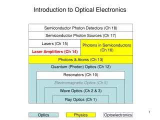
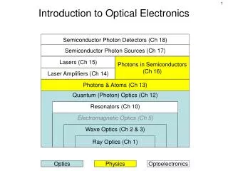
Semiconductor Photon Detectors (Ch 18). Semiconductor Photon Sources (Ch 17). Lasers (Ch 15). Photons in Semiconductors (Ch 16). Laser Amplifiers (Ch 14). Photons & Atoms (Ch 13). Quantum (Photon) Optics (Ch 12). Resonators (Ch 10). Electromagnetic Optics (Ch 5). Wave Optics (Ch 2 & 3).

Introduction to Optical Electronics
E N D
Presentation Transcript
Semiconductor Photon Detectors (Ch 18) Semiconductor Photon Sources (Ch 17) Lasers (Ch 15) Photons in Semiconductors (Ch 16) Laser Amplifiers (Ch 14) Photons & Atoms (Ch 13) Quantum (Photon) Optics (Ch 12) Resonators (Ch 10) Electromagnetic Optics (Ch 5) Wave Optics (Ch 2 & 3) Ray Optics (Ch 1) Optics Physics Optoelectronics Introduction to Optical Electronics
2 1 h h h E-field of Gaussian Beam Stimulated Emission Optics Ray Optics (Geometrical Optics) • Focus on location & direction of light rays • Limit of Wave Optics where 0 Wave Optics (Gaussian Beam) • Scalar wave theory (Single scalar wavefunction describes light) E&M Optics (Geometrical Optics) • Two mutually coupled vector waves (E & M) Quantum Optics (Photon Optics) • Describes certain optical phenomena that arecharacteristically quantum mechanical
Chronological Development of Optics • Euclid (300 BC) • Hero of Alexandria (150 BC – 250 AD ?) • Alhazen (1000 AD) • Franciscan Roger Bacon (1215 – 1294) • Johannes Kepler (1571 – 1630) • Willebrord Snell (1591 – 1626) • Rene Descartes (1596 – 1650) • Pierre de Fermat (1601 – 1665)
Simple OpticsSpherical Mirror Paraboloid • Rays parallel to and close to axis (paraxial) act like a paraboloid mirror • Parallel rays further from axis focus to caustic (green line) • The caustic is the surface perpendicular to all reflected parallel rays Spherical
Refraction & Total Internal Reflection Snell’s law of refraction: For Total Internal Reflection:
A y P1 C P2 F z1 -R z2 0 Concave & Convex Mirrors
Concave & Convex Mirrors(Paraxial Approximation) z1 -R z2 0 z1 0 z2 R
Spherical Boundaries Refraction y V P1 C P2 R
y O z z Spherical Boundaries Refraction
Thin Lenses y O F f O
Lenses • Bi-convex • R1 > 0 • R2 < 0 • Bi-concave • R1 < 0 • R2 > 0 • Planar Convex • R1 = ∞ • R2 < 0 • Planar Concave • R1 = ∞ • R2 > 0 • Meniscus Convex • R1 > 0 • R2 > 0 • R2 > R1 • Meniscus Concave • R1 > 0 • R2 > 0 • R1>R2
Ray Transfer Matrix (ABCD Matrix) A method for mapping rays through a series of optical elements. Assumes: • Paraxial approximation (slope = rise/run = tan ) • Linear relation between exit (y2, 2) and entrance (y1, 1) coordinates Output Plane Input Plane 2 where A, B, C and D are real. 1 y2 y1 Optic Axis z1 z2
ABCD MatrixExample: Free Space Output Plane Input Plane 2 y2 1 y1 Optic Axis d z2 z1
2 1 y1= y2 Optic Axis z1,2 ABCD MatrixExample: Refraction across planar boundary
Input Plane Output Plane 2 1 y1 y2 Optic Axis z2 z1 ABCD MatrixExample: Thin Lens
-R -R Concave Mirrors
Simple Optical Components Free-Space Propagation Refraction at a Planar Boundary Refraction as a Spherical Boundary convex, R>0; concave, R<0 Transmission Through a Thin Lens convex, f>0; concave, f<0 Refraction from a Planar Mirror Refraction from a Spherical Mirror convex, R>0; concave, R<0
d R2 R1 M1 M2 d d d Optical Cavities … Unit Cell
Explain these lens systems • Parallel rays entering the system all exit at the same y2 • Rays entering the system at the same point y1, all exit at y2. • Parallel rays enter system, emerging rays are also parallel • Rays emit from a single point, emerge parallel
Semiconductor Photon Detectors (Ch 18) Semiconductor Photon Sources (Ch 17) Lasers (Ch 15) Photons in Semiconductors (Ch 16) Laser Amplifiers (Ch 14) Photons & Atoms (Ch 13) Quantum (Photon) Optics (Ch 12) Resonators (Ch 10) Electromagnetic Optics (Ch 5) Wave Optics (Ch 2 & 3) Ray Optics (Ch 1) Optics Physics Optoelectronics Introduction to Optical Electronics
Chronological Development of Optics (part 2) • Robert Hooke (1635 – 1703) • Isaac Newton (1642 – 1727) • Christian Huygens (1629 – 1695) • Thomas Young (1772 – 1829) • Augustin Fresnel (1788 – 1827) • Speed of Light • Christenson Romer (1644 – 1710) • Armand Fizeau (1819 – 1896) • Jean Bernard Foucault (1819 – 1868)
Wave Optics *A(r) varies slowly with respect to
Spherical Paraboloidal Plane Elementary Waves