Download
1 / 47
470 likes | 577 Views
Summer School on Ocean Observation with Remote Sensing Satellites 18-23 June 2010. Definition of data assimilation problem and some solutions. Lecturer: Srdjan Dobricic CMCC, Bologna. Statistical background (model and observational spaces).

E N D
Summer School on Ocean Observation with Remote Sensing Satellites 18-23 June 2010 Definition of data assimilation problem and some solutions Lecturer: Srdjan Dobricic CMCC, Bologna
Statistical background (model and observational spaces) - Model state vector (may contain all model points – im*jm*km*param) - Observational state vector
Statistical background (introduction) The model state vector has the temporal dimension which spans the analysis window: xk x1 x0
Statistical background (introduction) The observational vector also has the temporal dimension which spans the analysis window: yk y1 y0
Statistical background (introduction) Model and observational spaces are connected by the observational operator H (non-linear): It is assumed that the modelled process is of the Markov type: - Model operator (non-linear) Compare to: Model dynamical operator (non-linear)
Statistical background (introduction) The posterior conditional pdf of the inverse solution is given by: - Probability density of observations given the model state - Probability density of the model estimate - Observational state vector - Model state vector
Definition of cost function (Gaussian model)
Definition of cost function (Gaussian model) The most likelyhood model state is the one which gives the maximum of:
Definition of cost function (Gaussian model) At this point the magnitude of the exponent has the minimum value. Therefore, in order to find the most likelyhood model state vector we must find the minimum of the following cost function:
Definition of cost function (Gaussian model) Errors Errors contain observational errors and “representativnes” errors
Definition of cost function (Gaussian model) - a priori information on model parameters. It can be any reasonable a priori estimate.
Definition of error covariances (Gaussian model) Errors are erros of the initial state estimate Errors and/or are model erros Is there some other way to define a priori model state estimate?
Definition of error covariances (Gaussian model) C - covariances of model state errors B0- covariances of initial model state errors Q - covariances of model errors A - covariances between initial model state errors and model errors
Definition of error covariances (Gaussian model) Now, in order to simplify the mathematics, we may assume that A=0: We assume that errors of initial state are independent from model errors Can we do that?
Definition of error covariances (Gaussian model) If A=0 the cost function becomes:
Definition of cost function (Gaussian model) We can further simplify the cost function by assuming a special structure of error covariances in Q. Often it is assumed that model errors are uncorrelated in time (unbiased):
Definition of cost function (Gaussian model) We can also assume a special structure of error covariances in R. Often it is assumed that observational and representativnes errors are uncorrelated in time (unbiased):
Definition of cost function (Gaussian model) In this case the cost function becomes: What is the best definition of a priori model state estimates ?
Definition of cost function (Gaussian model) If: If:
Definition of cost function (Gaussian model) Another simplification of the cost function is made by the assumption that model errors are temporally constant. In this case we can write: The cost function becomes:
Definition of 4D-VARcost function Furthermore, we can simplify the cost function by assuming that the model is perfect: The cost function becomes: Usually in the meteorological and oceanographic literature this cost function is named 4D-VAR. The assumption of the perfect model is implicitly assumed.
Minimization of 4D-VARcost function: Newton method The zero of a function can be efficiently found using the gradient. f(x) x3 x2 x1 x At the minimum the gradient of the cost function g(x) is equal to zero.
Minimization of 4D-VARcost function: Quasi-Newton and conjugate gradient methods In the quasi-Newton method the second derivative of J is approximated by symmetric positive definite matrices which are updated in each iteration of the minimizer by a symmetric update: In the conjugate gradient method the second derivative of J is estimated by using orthogonal directions. Again we need the information about the gradient of J. There is a freely available software package which applies BFGS formula with the limited computer memory (RAM).
Tangent linear approximation Observational operator Small perturbation H H H(x) x xk (Xk+p)
Tangent linear approximation Observational operator:
Tangent linear approximation Model operator
Minimization of 4D-VARcost function Variable transformation
Minimization of 4D-VARcost function Iterations of the minimizer • Calculate cost function • Calculate the gradient • Update the second derivative estimate • Estimate the next model state vector • If the gradient is sufficiently small stop There are freely available software packages to do this
Steps in minimization of cost function 1. Calculate misfits dk in a single run of the non-linear model fron time 0 to time n. 2. Start minimization by setting v=0. In the first step the cost function is just a veighted sum of squares of misfits:
Steps in minimization of cost function (incremental method) 3. In each following step calculate the cost function and the gradient: 3.1: Space transformation (model of B0) 3.2: Model integrationfrom 0 to k (single run) Mapping to observational space 3.3: Transform from observational to model space 3.4: Integration from k to 0 by the adjoint (single run). At time step n all adjoint variables are initialized by 0. At each time step they are forced by contributions from misfits. 3.5: Transform back to control space 3.6:
Steps in minimization of cost function 4. Linearize the model around the best estimate of the model trajectory and repeat steps 1-3.
Analysis error covarinace matrix The Hessian of the cost function is: We will show that the analysis error covariance matrix is the inverse of the Hessian of the cost function. The gradient will be written in the following way:
Analysis error covarinace matrix The terms in the gradient of the cost function from the previous equation can be rearranged in the following way: Multiplying the left and the right sides by their respective transposes gives:
Analysis error covarinace matrix We assumed that and From definitions: It follows that
Advantages and disadvantages of 4D-VAR • Advantages: • In the case of the perfect linear model 4D-VAR gives the model state estimates which are equivalent to Kalman smoother estimates • This is achieved at a smaller computational cost than with the full Kalman smoother algorithm • Outstanding problems: • If the model is non-linear the computationally efficient incremental solution is accurate only on short time windows. • The inclusion of the model error complicates the algorithm significantly • The analysis error covariance matrix is available only at the beginning of the assimilation window (quite useless)
3D-VARcost function 3D-VAR is an approximation of 4D-VAR in which it is assumed that the model that propagates background error covariances is the identity matrix. Therefore the assimilation window has to be adequately short.
Advantages and disadvantages of 3D-VAR (in comparison to 4D-VAR) • Advantages: • It is computationally much cheaper • The non-linearity is a less important problem, because the model trajectory is corrected in each step • Outstanding problems: • 3D-VAR is a filter • The background error covariance matrix is not optimally estimated
Definition of Kalman Filter (Gaussian model)
Relationship to variational methods • If the model error is uncorrelated in time Kalman filter and linear 4DVAR with an imperfect model give the same model state estimate at the end of the time window. • 4DVAR is a smoother: It estimates all model states by considering all observations. • Kalman filter is very simple to apply when the model state is small. • The ensemble Kalman filter is an approximation of the Kalman filter which uses an ensemble (typically small) of forecasts and analyses in order to approximate the full dimension of Kalman filter matrices
Relationship to variational methods • OI gives the same solution as 3DVAR • An advantage is the simplicity of equations • A disadvantage is the limited application to simple observational operators and error covariance models, because it requires the inversion of matrices • Again, the ensemble method may simplify the calculus
Suggested literature • Boutier, F., and P. Courtier, 1999. Data assimilation concepts and methods, ECMWF report. (available from www.ecmwf.int) • Lewis, J., S. Lakshmivarahan, and S. Dhall, 2006: Dynamic Data Assimilation, Cambridge Univ. Press, 654 pp.