Download
1 / 36
360 likes | 490 Views
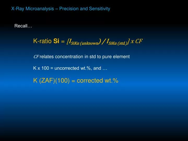
X-Ray Microanalysis – Precision and Sensitivity. Recall… K-ratio Si = [ I SiK α (unknown ) / I SiK α (std.) ] x CF CF relates concentration in std to pure element K x 100 = uncorrected wt.%, and … K (ZAF)(100) = corrected wt.%. Precision, Accuracy and Sensitivity (detection limits).

E N D
X-Ray Microanalysis – Precision and Sensitivity Recall… K-ratio Si = [ISiKα (unknown) / ISiKα (std.)] x CF CF relates concentration in std to pure element K x 100 = uncorrected wt.%, and … K (ZAF)(100) = corrected wt.%
Precision, Accuracy and Sensitivity (detection limits) Precision: Reproducibility Analytical scatter due to nature of X-ray measurement process Accuracy: Is the result correct? Sensitivity: How low a concentration can you expect to see?
Accuracy and Precision Measured value Ave Std error Standard deviation Ave Std error 20 25 30 35 20 25 30 35 Correct value Correct value Wt.% Fe Wt.% Fe Low precision, but relatively accurate High precision, but low accuracy
Ave Std error Ave Std error Accuracy and Precision Measured value Ave Std error Standard deviation 20 25 30 35 20 25 30 35 Correct value Correct value Wt.% Fe Wt.% Fe Low precision, but relatively accurate High precision, but low accuracy Precise and accurate
Characterizing Error • What are the basic components of error? • Short-term random error (data set) • Counting statistics • Instrument noise • Surface imperfections • Deviations from ideal homogeneity • Short-term systematic error (session to session) • Background estimation • Calibration • Variation in coating • 3) Long-term systematic error (overall systematic errors that are reproducible session-to-session) • Standards • Physical constants • Matrix correction and Interference algorithms • Dead time, current measurement, etc.
Short-Term Random Error - Basic assessment of counting statistics X-ray production is random in time, and results in a fixed mean value – follows Poisson statistics At high count rates, count distribution follows a normal (Gaussian) distribution Frequency of X-ray counts Counts
99.7% of area 95.4% of area 68.3% of area The standard deviation is: 3σ 2σ 1σ 1σ 2σ 3σ
Variation in percentage of total counts = (σC / N)100 So to obtain a result to 1% precision, Must collect at least 10,000 counts
Evaluation of count statistics for an analysis must take into account the variation in all acquired intensities Peak (sample and standard) Background (sample and standard) And errors propagated Addition and subtraction Relative std. deviation Multiplication and division
i Current from the Faraday cup tp Counting time on the peak r+ et r- Positive and negative offsets for the background measurement, relative to the peak position Total counting time tb P Peak counts Background counts B Cs Element concentration in the standard s Intensity (Peak-Bkgd in cps/nA) of the element in the standard Ce Element concentration in the sample e Intensity (Peak-Bkgd in cps/nA) of the element in the sample jp, jb index of measurements on the peak and on the background jpmax, jbmax Total number of measurements on the peak and on the background
For the calibration… And standard deviation…
The measured standard deviation can be compared to the theoretical standard deviation … Theo.Dev(%) = 100* Stheo/s The larger of the two then represents the useful error on the standard calibration: ²s = max ((Smeas)², or (Stheo)²)
For the sample, the variance for the intensity can be estimated as… where
The intensity on the sample is… Or, in the case of a single measurement… Pk – Bkg cps/nA
An example Calibration
Sample Th data Wt% curr pk cps pk t(sec) bkg cps pk-bk 6.4992 200.35 4098.57 800 285.0897 3813.483 This is a very precise number
Sensitivity and Detection Limits Ability to distinguish two concentrations that are nearly equal (C and C’) 95% confidence approximated by: N = average counts NB = average background counts n = number of analysis points Actual standard deviation ~ 2σC, so ΔC about 2X above equation If N >> NB, then
Sensitivity in % is then… To achieve 1% sensitivity Must accumulate at least 54,290 counts As concentration decreases, must increase count time to maintain precision
Example gradient: Wt% Ni 0 distance (microns) 25 Take 1 micron steps: Gradient = 0.04 wt.% / step Sensitivity at 95% confidence must be ≤ 0.04 wt.% Must accumulate ≥ 85,000 counts / step If take 2.5 micron steps Gradient = 0.1 wt.% / step Need ≥ 13,600 counts / step So can cut count time by 6X
Detection Limits N no longer >> NB at low concentration What value of N-NB can be measured with statistical significance? Liebhafsky limit: Element is present if counts exceed 3X precision of background: N > 3(NB)1/2 Ziebold approximation: CDL > 3.29a / [(nτP)(P/B)]1/2 τ = measurement time n = # of repetitions of each measurement P = pure element count rate B = background count rate (on pure element standard) a = relates composition to intensity
Or 3.29 (wt.%) / IP[(τ i) / IB]1/2 IP = peak intensity IB = background intensity τ = acquisition time i = current Ave Z = 79 Ave Z = 14 Ave Z = 14, 4X counts as b
Detection limit for Pb PbMα measured on VLPET 200nA, 800 sec
Can increase current and / or count time to come up with low detection limits and relatively high precision But is it right?
Accuracy All results are approximations Many factors Level 1 quality and characterization of standards precision matrix corrections mass absorption coefficients ionization potentials backscatter coefficients ionization cross sections dead time estimation and implementation Evaluate by cross checking standards of known composition (secondary standards)
Level 2 – the sample Inhomogeneous excitation volume Background estimation Peak positional shift Peak shape change Polarization in anisotropic crystalline solids Changes in Φ(ρZ) shape with time Measurement of time Time-integral effects Measurement of current, including linearity is a nanoamp a nanoamp? Depends on measurement – all measurements include errors!
Time-integral acquisition effects drift in electron optics, measurement circuitry dynamic X-ray production non-steady state absorbed current / charge response in insulating materials beam damage compositional and charge distribution changes surface contamination
Overall accuracy is the combined effect of all sources of variance…. σT2 = σC2+σI2+σO2+σS2+σM2 σT= total error σC= counting error σI= instrumental error σO= operational error σS= specimen error σM= miscellaneous error Each of which can consist of a number of other summed terms Becomes more critical for more sensitive analyses - trace element analysis
Sources of measurement error – Time-integral measurements and sample effects
2σ counting statistics Cps/nA 0 5 10 15 20 25 30 Time (min)
Cps/nA Wavelength (sinθ)
Sources of measurement error: Extracting accurate intensities – peak and background measurements Background shape depends on Bremsstrahlung emission Spectrometer efficiency